Decision Support for a Centre Pivot Irrigation System Based on Numerical Modelling

Decision Support for a Centre Pivot Irrigation

System Based on Numerical Modelling

Andrei-Mugur Georgescu

1

, Remus Alexandru Madularea

2

, Petre-Ovidiu

Ciuc

2

and Sanda-Carmen Georgescu

2*

1

Technical University of Civil Engineering Bucharest, Bucharest, Romania 2_{University “Politehnica” of Bucharest, Bucharest, Romania}

[email protected], [email protected], [email protected], [email protected]

Abstract

We focus on the operation of a real centre pivot irrigation system. The system encountered problems in 2016 and did not operate for several weeks due to the low level of the Danube (its water source). In that period, water level in the Danube went below the most probable minimal level during summer, with a return period of 30 years. With a natural desire to solve the problem, the owner of the system added a new pump near the water intake. This new, double-entry vertical axis pump, coupled in series with the existing pumping station situated further downstream, added roughly 1 bar to the pressure in the system. Things went well till the end of summer 2017 when, due to a pressure surge in the pumping station (most likely at shutoff head), one of the anti-vibration joints detached suddenly from the discharge pipe, and the pumping station was entirely flooded. The performed analysis helped understand the reasons of the accident and provided solutions (including pumping operating rules and schedule for pivots that can be operated simultaneously) that will hopefully avoid reoccurrences in the future, without affecting the day to day operation of the system.

1

Introduction

In this paper, we focus on the operation of a new centre pivot irrigation system, located in Romania (at Seimenii Mici), in the Dobrogea region (between the Danube river and the Black Sea, about 9 km away from the Nuclear Power Plant of Cernavoda).

The centre pivot is a method of irrigation based on the rotation of equipment around a pivot. The crops are watered by overhead sprinklers mounted on the equipment, thus, a circular area centred on the pivot is irrigated [1,2]. In order to avoid unbalanced watering of the crops, a pressure reducing

* _{Corresponding author}

Engineering

Volume 3, 2018, Pages 764–771

valve is mounted before each sprinkler. Equipment’s rotation around the pivot is usually propelled by electric motors. Such systems are considered to be highly efficient and use less water than other surface irrigation systems. The pivot itself is just a vertical pipe coming out of the ground and supplying the sprinklers of the equipment. Within a hydraulic analysis, modelling the pivot as a simple nozzle, i.e. an uncontrolled orifice, where the discharge depends on the pressure [3], is not representative for the real behaviour of the system. Of course the multitude of sprinklers supplied by the pivot can be modelled as a single "bigger" orifice (its outflow coefficient can be computed based on pivot's technical specifications, namely the nominal flow rate and the pressure requested for full service), but a pressure reducing valve should also be inserted before the orifice to avoid the increase of flow rate in case of exceeding pressure. Such a behaviour fits the pressure-driven simulation models. Pressure-driven analysis can be directly performed in software like Bentley WaterGEMS, WDNetXL [4], WaterNetGen [5] and others. Demand-driven simulation models are not primarily fit for uncontrolled discharge orifices. Although EPANET allows performing mainly demand-driven analysis, it also incorporates emitters that model pressure-dependent outflow at orifices [6] and pressure reducing valves. Being a free software and due to its versatility, EPANET was thus the preferred choice for the analysis presented in this paper.

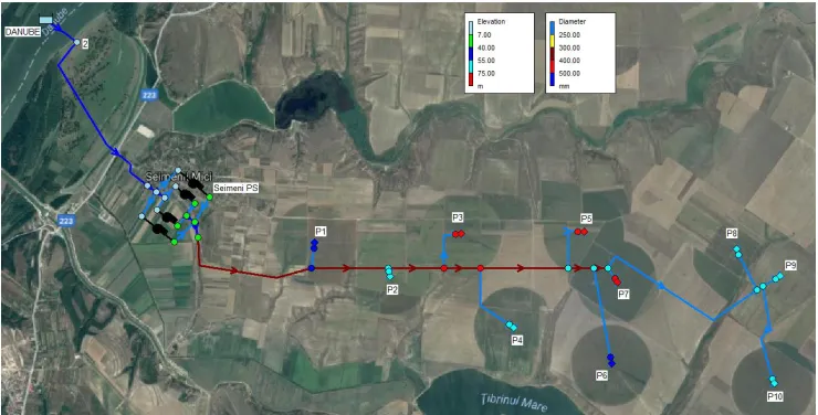
The model of the irrigation system consists of 10 identically equipped centre pivots, supplied with water pumped from the Danube, through a branched network. The total cumulated length of the pipes in the system is of 16.25 km. Each pivot must be able to supply a flow rate of about 55 l/s at 3 bar (minimum 2.6 bar) for the correct operation of the equipment. A scheme of the irrigation system with elevations (from 3.5 m to 88 m) and pipes' inner diameters (from 200 mm to 582 mm) is presented in figure 1, superposed on a Google map screen shot of the area.

Figure 1: Hydraulic scheme of the centre pivot irrigation system  configuration : water source (Danube), Seimeni PS and 10 pivots (P1 to P10); elevations [m] and diameters [mm] are displayed using colour bars

The irrigation system built based on the above design configuration, termed further as configuration  (figure 1), was commissioned in the spring of 2016 and used during the summer of 2016. Unfortunately, in the summer of 2016, the Danube level decreased to a level below the minimal design limit and the system had to be stopped frequently, due to unusual vibrations and noises in the pumping station (at times, pumps' rotors ran with cavitation on their suction side, but saving the crops prevailed over protecting the rotors). Obviously, insufficient watering of the crops also occurred.

To avoid future problems related to cavitation of pumps and to water shortage (when Danube’s level will get lower than the minimal design value), by the end of 2016, the owner of the irrigation system installed an additional pump (double-entry vertical axis pump, variable speed driven) on the intake pipe, located at node 2, near the Danube (figure 1)  the new configuration of the system will be termed further as configuration . Within the configuration , during the summer of 2017, Seimeni PS became a second stage PS, operating in better conditions than in the previous year.

The overpressure of about 1 bar, induced by the double-entry pump from node 2, pushed the system near its upper pressure limit on the discharge pipes of pumps from Seimeni PS (pipes with PN16 nominal pressure). In September 2017, due to a pressure surge at one pump (most likely at shutoff head), the anti-vibration joint detached suddenly from the discharge pipe, the Seimeni Pumping Station was entirely flooded, and equipments were severely damaged. Following that event, the owner requested a solution for refurbishing Seimeni PS with minimal costs.

In order to understand the reasons of the accident, and to analyse the refurbished system within the configuration , EPANET numerical models for both configurations  and  were built, based on the methodology presented in Section 2. Further, in Section 3, the results were compared, and finally a decision support tool, including safety pumping operating rules and a schedule for pivots that can be operated simultaneously within the configuration  was provided.

2

Methodology

An EPANET model of the irrigation system was built for the configuration  (figure 1). As mentioned above, the pivot can be modelled as a nozzle, where the discharge Q_n is defined upon the

full service pressure p_n, namely: Qnap0n.5, where the value of the outflow coefficient (emitter

coefficient in EPANET) results a9.94103 m2.5/s, at the nominal flow rate of the considered pivot:

3

10 44 .

54  



n

Q m3/s. Before each pivot, a pressure reducing valve keeps the downstream pressure at

30 

n

p mWG (about 3 bar), when the upstream pressure is above that limit.

Several simulations with different conditions were performed for the configuration  of the system. It turned out that some combinations of pivots could not ascertain the requested flow or pressure requirements, resulting in improper irrigation of the crops, even at design level of the Danube. Subsequently, a more thorough analysis of all the possible combinations of 3 pivots out of the existing 10 was performed. This analysis assumed that all 3 pivots operate at nominal conditions and that all 3 (identical) centrifugal pumps of the PS are working at nominal speed. With this assumption, the flow through one pump must equal the requested flow of one pivot; hence the head given by a pump at the nominal flow rate of one pivot can be directly obtained from the pump curve. The head versus flow rate curve of the pumps from Seimeni PS, constructed at nominal speed and introduced in the EPANET model, is presented in figure 2.

The available specific energy (available head) of the system, H_A (measured in [m]), is computed

as the sum between the level of water in the Danube and the pumping head: H_Az_DH_p, where

D

pump working at a flow rate equal to the nominal flow rate of the pivot. From the pump curve, the resulting pump head is H_p 149.7 m (see the operation point in figure 2). The discharge pressure of pumps in Seimeni PS reaches 151.6 mWG for the configuration  (meaning that the pressure is below, but quite closed to the admissible PN16 level).

Figure 2: Head versus flow rate curves of pumps in Seimeni PS, at nominal speed (speed factor 1) and at speed factors 0.98 and 0.973; operation point for configurations  and  at nominal speed;

operation points for configuration  at 0.98 and 0.973

The necessary specific energy (necessary head) of the system, H_N (in [m]), is computed as the maximum value of the sum between the necessary head of each pivot and the corresponding head losses in the system, for each combination of 3 operating pivots, as:

}

{

D P

; ;

) (

max _{n n r n}

k j i n

N z p g h

H _

  

  , (1)

where n



i; j;k



represent the indexes of the 3 operating pivots, z_n represents the ground elevation

at the location of pivot P_n, the pressure head p_n (



g)30 m ( is the water density and g the

gravity), and

n r

hDP is the value of head losses on the path from the Danube up to the pivot Pn. The

head losses can be expressed as: _ 



_{m m m}

n

r R Q

hD P ( 2), where m is the index of the pipes between

Danube and the pivot P_n; R_m is the hydraulic resistance of the pipe (measured in [s2/m5]); Q_m is the flow rate through the pipe of index m; the roughness was set on each pipe (from 2 mm on the intake pipe, to 0.1 mm on pipes connected to pivots); the Darcy-Weisbach friction factor was computed using the Swamee and Jain formula [7]. Minor losses on pipes, as well as inlet and outlet kinetic terms, were neglected.

Going back to figure 1, we notice that, for any combination of 3 operating pivots, the flow rate through the main pipes between the Danube (inlet) and the ramification of the first pivot equals 3Q_n. The flow through the ramification of each pivot, as well as the flow rate through the pipes that couple the pumps to the mains is always equal to Q_n. This leaves only the pipes between the ramification of

the first pivot to the ramification of the pivot P8 that can experience either Q_n, 2Q_n or 3Q_n, depending on the combination of operating pivots. This observation reduces drastically the calculations (number of EPANET runs) required in order to ascertain the head losses on the pipes for

0 20 40 60 80 100 120

80 90 100 110 120 130 140 150 160 170

flow rate [l/s]

pum

p

he

ad

[m

]

Q

n = 54.44 l/s

pump curve at nominal speed

pump curve at  = 0.98

pump curve at  = 0.973

operation point at nominal speed

operation point,  = 0.98

all 120 possible combinations. An MS Excel spread sheet was used subsequently, in order to calculate the sums of the head losses for all the possible combinations of 3 pivots.

Finally, the available specific energy and the necessary specific energy were compared. As long as the necessary specific energy was below the available one, H_NH_A, the combination of operating pivots was marked as feasible. Otherwise, the combinations could not be realized.

The solution obtained for the system with configuration , denoted further as solution , provided a schedule for pivots that can be operated simultaneously in the given conditions.

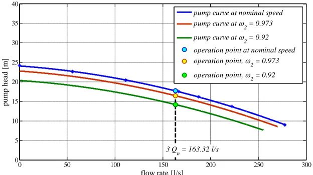
As already mentioned, in order to improve the overall system operation, an additional pump was connected in node 2 on the intake pipe (figure 1), leading to the configuration  of the system. To analyse the refurbished system, we modified the EPANET model built for the configuration , and obtained a model for the refurbished configuration . The head  flow rate curve of the additional pump, at nominal speed, inserted in the second EPANET model, is shown in figure 3.

Figure 3: Head versus flow rate curves of the additional pump in node 2, within the configuration , at nominal speed (speed factor ₂1), at speed factors ₂0.973 and ₂0.92, and operation points

The same specific energy analysis was performed for the new configuration, by simply adding to the available specific energy, the head H_p2 provided by the additional pump at a flow rate of 3Q_n,

that is: H_AzDH_p2H_p. If all pumps are running at their nominal speed within the configuration

, from the pump curves (figures 2 and 3), the operation points result: {3Qn 163.32103 m 3

/s;

69 . 17

2 p

H m} for the additional pump in node 2, and {Q_n 54.44103 m3/s; H_p149.7 m} for each of the 3 working pumps in Seimeni PS. The discharge pressure of pumps in Seimeni PS reaches 161.83 mWG for the configuration  (meaning that the pressure is above the admissible PN16 level). The solution, denoted further as solution , reduced considerably the number of unavailable combinations of 3 pivots, but the discharge pressure is dangerously high in Seimeni PS.

In order to decrease the discharge pressure of pumps in Seimeni PS, the obvious choice, ensuring safety in operation, is to set a lower speed for the working pumps within the configuration .

The head  flow rate curves were derived for each pump, based on affinity laws, as second order polynomial regressions, with speed factor  and



₂ respectively as parameter. Thus, the resulting

curves, HH



Q,





for pumps in Seimeni PS and H₂H₂



Q₂,



₂



for the additional pump in node

0 50 100 150 200 250 300

0 5 10 15 20 25 30 35 40

flow rate [l/s]

pum

p

he

ad

[m

]

3Q

n = 163.32 l/s

pump curve at nominal speed

pump curve at 

2 = 0.973

pump curve at 

2 = 0.92

operation point at nominal speed

operation point, 

2 = 0.973

operation point, 

2 were: H157.8920.16103Q2.76103Q2; 22 3 2

2 2

2

2 24.09 0.018 Q 0.13 10 Q

H       

with pumping heads in [m], for flow rates in [l/s].

As stated before, the flow rate value attached to the operation point was imposed for each working pump, namely: QQ_n for 3 pumps in PS, and Q₂3Q_n for the pump in node 2. Moreover, to minimize the energy consumption, all 3 pumps in PS must work at the same speed factor [8].

The pumping schedule related to speed factors was derived in GNU Octave [9], as a solution of the nonlinear system of equations describing the operation of the hydraulic system, containing mass balance equations in nodes and energy balance equations on pipes, on the path from Danube, to the discharge section (DS) of pumps in Seimeni PS. The pressure head at the discharge section of pumps in PS is denoted by H_DSp_DS (



g).

Taking into account the fact that within the PS, pumps are mounted on similar hydraulic circuits (leading to the same head losses between the PS inlet and the discharge section of each pump), and that all 3 pumps have identical operation points, the above system of equations reduces to a single equation, as:



2







DS DS D DS 2

DHp 3Qn, Hp Qn, z H hr 

z   , (2)

where z_DS is the elevation of the horizontal discharge section, and h_rDDS is the value of head losses on the path from the Danube up to the discharge section of a pump in PS. Equation (2) has 3 unknowns, namely the speed factors



₂ and , and the pressure head H_DS. Due to pipe pressure

limit (PN16), the following condition is added: H_DS160 m (an imposed constant value of H_DS can

be used further). Another condition must be defined for the speed factors, e.g.



₂



; or 1 (imposed value) and



₂ computed; or



₂1 and  computed. The new set of rules regarding the pumps operation yielded the third EPANET model.

3

Results and Discussion

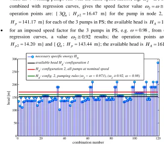
The resulting necessary total head H_N, for all 120 combinations of 3 pivots in simultaneous operation, for both configurations  (the initial one) and  (refurbished), is plotted in figure 4.

For the system within configuration , where all 3 pumps in Seimeni PS run at nominal speed, and the available head was H_A153.2 m, the solution  provided 72 feasible combinations of 3 pivots in simultaneous operation; thus, 48 out of the total of 120 combinations (i.e. 40%) do not meet the requirements  see figure 4, where H_N H_A153.2 m for 48 combinations.

For the system within configuration , where all 4 working pumps (one in node 2 and three in PS) run at nominal speed, and the available head is H_A170.9 m, the solution  reduced considerably the number of unavailable combinations of 3 pivots: only 21 out of 120 combinations (i.e. 17.5%) do not meet the requirements  see figure 4, where H_NH_A170.9 m for 21 combinations. From this point of view, the additional pump improved the operation of the system. Unfortunately, in this case, the discharge pressure is dangerously high in Seimeni PS (above the PN16 limit), so the solution  does not ensure safety in operation.

 when all 4 working pumps run with the same speed factors, e.g.



₂



, equation (2), combined with regression curves, gives the speed factor value



₂



0.973; the

operation points are: {3Q_n; Hp2 16.47 m} for the pump in node 2, and {Qn;

17 . 141



p

H m} for each of the 3 pumps in PS; the available head is H_A161.14 m;

 for an imposed speed factor for the 3 pumps in PS, e.g. 0.98, from (2) and the regression curves, a value



₂0.92 results; the operation points are: { 3Q_n ;

20 . 14

2 p

H m} and {Q_n; Hp 143.44 m}; the available head is HA161.14 m.

Figure 4: Necessary total head H_N for all 120 combinations of 3 working pivots out of the total 10 pivots,

and available head H_A, at the minimal design level of Danube (3.5 m), for configuration , and for configuration  where all pumps run at nominal speed, or pumps run under specified operation rules

Obviously, for a fixed H_DS value, the same H_A value results from calculations (the same value

of the sum between Hp2 and Hp), for different pumping rules. Other pumping rules can be selected,

e.g.



₂1 and  computed (where the resulting value is 0.969 ).

The solution , attached to the above pumping operating rules, yields 28 out of 120 combinations (i.e. 23.3%) that do not meet the requirements  see figure 4, where H_NH_A161.14 m for 28 cases. The solution  can be adopted as decision support, valid on short and medium term (up to the moment when the owner of the system will change all pipes on the discharge side of the PS with pipes of PN25 nominal pressure).

To exemplify the results, we present in figure 5 the flow rate distribution on pipes and pressure at nodes, for the operation of pivots P3, P5 and P10, within configuration , for



2



0.973.

4

Conclusions

In this paper, a centre pivot irrigation system, located in Romania, was modelled in order to get a decision support tool for the day to day operation of the system. The above mentioned tool includes a pumping schedule (via speed factors values) and a schedule for combinations of 3 pivots that can be

0 20 40 60 80 100 120

0 50 100 150 200 250 300

combination number

he

ad

[m

]

necessary specific energy H

N

available head H

A: configuration 1

H

A: configuration 2, all pumps at nominal speed

H

operated simultaneously. The proposed solution considered the previous problems encountered for that irrigation system. The solution was derived based on pressure restrictions imposed in the pumping station (to avoid reoccurrence of pressure surges), without affecting crops watering.

Figure 5: Flow rate on pipes (in [l/s]) and pressure in nodes (in [mWG]), displayed using colour bars, for the operation of pivots P3, P5 and P10, within configuration , for ₂0.973

References

[1] L. New, G. Fipps, Center pivot irrigation, Texas Agricultural Extension Service, The Texas A&M University System, B-6096, 2000.

[2] P. Smith, J. Foley, S. Priest, S. Bray, J. Montgomery, D. Wigginton, J. Schultz, R. Van Niekerk, A review of centre pivot and lateral move irrigation installations in the Australian Cotton Industry, New South Wales Department of Primary Industries, 2014.

[3] O. Giustolisi, T.M. Walski, Demand components in Water Distribution Network Analysis, J. Water Res. Pl.-ASCE, 138(4) (2012), 356–367.

[4] O. Giustolisi, D.A. Savić, L. Berardi, D. Laucelli, An Excel based solution to bring water distribution network analysis closer to users, in: D.A. Savić, Z. Kapelan, D. Butler (Eds.), Urban Water Management: Challenges and Opportunities, University of Exeter, vol. 3, 2011, pp. 805–810.

[5] J. Muranho, A. Ferreira, J. Sousa, A. Gomes, A. Sá Marques, Pressure-dependent demand and leakage modelling with an EPANET extension – WaterNetGen, Procedia Engineering, 89 (2014), 632–639.

[6] L. Rossman, EPANET 2 Users Manual, U.S. Environmental Protection Agency, EPA/600/R-00/057, Cincinnati, OH, 2000.

[7] P.K. Swamee, A.K. Jain, Explicit equations for pipe flow problems, J. Hydr. Eng. Div.-ASCE, 102(5) (1976), 657–664.

[8] S.-C. Georgescu, R. Popa, Application of Honey Bees Mating Optimization Algorithm to pumping station scheduling for water supply, U.P.B. Sci. Bull., Series D, 72(1) (2010), pp. 77–84.