INTEGRATING ANALYTICAL AEROELASTIC INSTABILITY ANALYSIS INTO DESIGN OPTIMIZATION OF AIRCRAFT WING
STRUCTURES
M. NIKBAY1, P. ACAR1§
Abstract. Two analytical flutter solution approaches have been developed to optimize two and three dimensional aircraft wing structures with design criteria based on aeroe-lastic instabilities. The first approach uses open loop structural dynamics and stability analysis for a two dimensional wing model in order to obtain the critical speeds of flutter, divergence and control reversal for optimization process. The second approach involves a flutter solution for three dimensional wing structures by using assumed mode technique and is applied to aeroelastic optimization based on flutter criterion efficiently. This flut-ter solution employs energy equations and Theodorsen function for aerodynamic load calculation and is fully-parametric in terms of design variables which are taper ratio, sweep angle, elasticity and shear modulus. Since bending and torsional natural frequen-cies are required for flutter solution, a free vibration analysis of aircraft wing is developed analytically as well. The analytical results obtained for flutter solution of AGARD 445.6 wing model for Mach number of 0.9011 are found to be compliant with the experimental results from literature. Next, the three dimensional flutter code is coupled with opti-mization framework to perform flutter based optiopti-mization of AGARD 445.6 to maximize the flutter speed.
Keywords: Aeroelasticity, flutter, divergence, control reversal, aeroelastic optimization.
AMS Subject Classification: 74F10, 90C31
1. Introduction
Aeroelasticity, as a multidisciplinary research field, investigates the behavior of an elastic structure in airstream and interaction of inertial, aerodynamic and structural forces. The static aeroelastic phenomena involve divergence and control reversal while flutter is a dynamic instability.
Theoretically, divergence happens when the twist angle of the root of the wing goes to infinity. By considering a more realistic approach, divergence is seen for large values of twist angle. Control reversal, which is also a static aeroelastic phenomenon, affects the expected behavior of the control surfaces of a wing and results with reverse functioning of the control surfaces. This has an influence on the maneuverability and stability of the aircraft.
1
Istanbul Technical University, Faculty of Aeronautics and Astronautics, Astronautical Engineering Department, Maslak, Istanbul, 34469, Turkey,
e-mail: [email protected] and [email protected]
§ Manuscript received 01 September 2011.
TWMS Journal of Applied and Engineering Mathematics Vol.1 No.2 cI¸sık University, Department of Mathematics 2011; all rights reserved.
The most catastrophic aeroelastic phenomenon, flutter, happens when the structure ex-tracts energy from air stream and can cause various types of damages to an aircraft struc-ture. Failure of the structure is even a possible case during flutter motion. Thus, flutter phenomenon must be taken into account in order to prevent possible harms. Therefore, determination of flutter speed with respect to related flight conditions is an indispensable process for aeroelasticians. Prediction of flutter can be achieved by several methods such as analytical, experimental and numerical approaches. Analytical solutions are the bases of modern numerical calculations and they follow required steps to understand the physical background of a dynamic aeroelastic system. Shubov [1], [2] states that the physical mean-ing of flutter can not be completely understood unless an analytical solution procedure is applied. Both experimental and numerical studies do not provide sufficient knowledge to understand the full physical meaning.
An analytical flutter solution for a wing model can be ”time or frequency based”, or another possibility is to define the related system in ”Laplace domain”. Time based ap-proaches are known as ”Time Marching Methods” which are based on a coupled form in-cluding correct estimations in both aerodynamics and structural displacements [3]. Laplace domain based studies provide a solution independent from time terms such that algebraic equations are adequate to find flutter speed [4]. These algebraic solutions can form an eigenvalue problem as in the study of Murty [5]. Another Laplace domain based solution procedure includesµ-p method which determines extreme eigenvalues that specify flutter boundaries [6]. Eller [7] makes use of linearization and defines the aerodynamic forces in terms of Laplace variable.
Frequency based flutter solution that has extensive application areas is chosen for three dimensional flutter analysis in the present work. Frequency based studies are traditional in the topic of dynamic aeroelasticity and they consist of well-known methods such as V-g and p-k. These approaches can also be used to obtain the flutter speed in transonic regimes [8]. Another frequency method, known as g method, stated by Ju and Qin [9], includes the contribution of Laplace variable. Several approaches can be obtained to define the aerodynamic forces in flutter solution such as Wagner Function, Theodorsen Function, Rational Function Approach and Indicial Function Approach.
In the present study, firstly a solution based on stability analysis to determine the speeds of divergence, control reversal and flutter in a two dimensional wing model is obtained via a developed Matlab code. The code is implemented into the optimization driver, Modefrontier for the multi-objective aeroelastic optimization. The solution procedure in two dimensional system forms a basis for a more realistic aeroelastic analysis and optimization in three dimensional structures.
An aeroelastic solution procedure based on assumed mode technique is applied to two benchmark problems and a realistic wing structure, AGARD 445.6 wing. The methodology stated in this work is the first and only analytical flutter solution attempt in literature for AGARD 445.6 wing to the best of authors’ knowledge. The starting point is the traditional Lagrange equations. The solution steps include definitions of structural parameters and inertia terms, use of Theodorsen aerodynamics for inviscid, incompressible and subsonic flight regime. Theodorsen aerodynamics provide an adaptable solution with frequency domain. Analytical approach can derive a parametrical solution as a tool for flutter based optimization.
2. Aeroelastic Analysis for Two Dimensional Wing Structures
An analytical solution procedure based on state-space representation of the related dynamic system and stability analysis are applied to a two dimensional wing structure in order to examine aeroelastic instabilities as flutter, divergence and control reversal. The solution forms a basis for aeroelastic analysis of more realistic wing configurations.
Formulation of the aeroelastic problem process includes convenient use of Lagrange and energy equations in order to obtain necessary equations of motion for two dimensional wing structure. The derived formulation can be used for divergence, control reversal and flutter instabilities since it is based on control approach. A suppressing control approach for aeroelastic effects contains two main phases as the determination of open loop dynamic characteristics and the design of compensator. Determination of open loop dynamic char-acteristics step is based on obtaining the region or speed in which an instability happens and it provides a solution for divergence, control reversal and flutter as aeroelastic insta-bilities.
The wing profile is modeled by using linear and torsional springs. Equations of wing motion that describe both plunging and pitching are derived from Lagrange equations. Lagrange equations can be written in a form as shown below:
d dt
∂T ∂q˙i
−
∂T ∂qi
+
∂V ∂qi
=Qi (1)
where T and V denote kinetic and potential energies while q and Q are generalized coordinates and forces.
Generalized forces in Lagrange equations include aerodynamic terms that can vary according to the flight regime at interest. In this section, aerodynamic forces for lift and pitching moment are obtained for inviscid, incompressible and quasi-steady case.
In the presence of control surfaces in both trailing and leading edge of the airfoil, the aerodynamic lift and pitching moment can be defined as follows:
L=−ρ∞U2bCLββ−ρ∞U
2bC
Lξξ−ρ∞U
2bC
Lα(α+α0) (2)
My =ρ∞U2b2CMββ+ρ∞U
2b2C
Mξξ+ρ∞U
2b2C
Mα(α+α0) (3)
where ρ∞ and U are free-stream density and velocity. b is half chord distance while
α, β and ξ denote deflections in pitching, trailing edge and leading edge control surfaces respectively. α0 shows the initial deflection of pitching. Aerodynamic lift coefficientsCLα,
CLβ,CLξ and moment coefficients CMα,CMβ,CMξ are defined for related deflections.
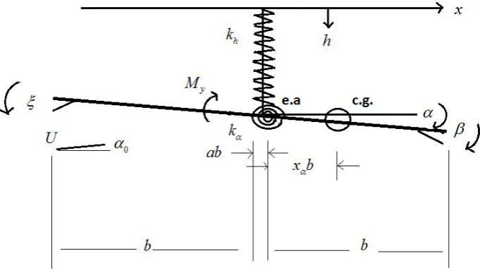
The solution can be applied to a wing section as shown in Figure 1 [11].
Figure 1 shows the modeling of wing motion with linear and torsional springs. The springs with coefficientskh and kα represent plunging and pitching motions respectively
whileβ and ξ are again the deflections of control surfaces.
Equations of wing motion for a two dimensional wing structure are obtained by consid-ering the section geometry above and using basic kinetic and potential energy equalities in Lagrange equation:
m¨h+mbxαα¨+khh=L(t) (4)
mbxαh¨+Iαα¨+kαα=My(t) (5)
In (4) and (5), hindicates plunging deflection whilemis mass of the airfoil,xαis static
Figure 1. Typical Section Geometry of Two Dimensional Wing Structure
The solution is based on utilization of open loop characteristics of dynamic systems. Therefore, it is more practical to define the system of equations with Laplace variables. Time dependent terms have to be transformed into Laplace domain to obtain algebraic equations.
h(t)→h(s) (6)
α(t)→α(s) (7)
¨
h(t)→s2h(s)−sh(0)−h(0)˙ (8)
¨
α(t)→s2α(s)−sα(0)−α(0)˙ (9) Assuming that all displacements and their derivatives in initial case are zero, final equa-tions of motion in Laplace domain are obtained for an aeroelastic stability analysis. The aeroelastic system is defined with respect to state-space representation. The characteristic equation, C(s), is obtained by using the necessary condition for the stability analysis as: det(sI−A) = 0 for a system in the following form where [A] indicates the state matrix:
s2¯h(s) s2α(s)
= [A]2×2
¯
h(s) α(s)
The effects of control surfaces have to be considered in the solution of control reversal phenomenon. Thus, the system of equation has to be re-arranged in a state-space form as :
s2¯h s2α
= rα2
C(s)
T11 T12 T13 T14 T21 T22 T23 T24
¯ h α β ξ
where Tij (i=1 to 2 and j=1 to 4) shows the transfer functions related to aeroelastic
phenomena,rα is radius of gyration and dimensionless plunge deflection is denoted by ¯h.
Tij is a transfer function including effects ofith term as output andjth term as input.
The reduced speed value for control reversal can be obtained by using T13 ( Thβ) since
Thβ indicates the stability of h displacement affected by control surface displacement in
trailing edgeβ within the context of control reversal phenomenon. The definition of T13 is given by [11] where ¯q indicates normalized dynamic pressure:
T13= ¯qCLβ
¯ qCMα
1− CLαCMβ
CMαCLβ
−1−s2
1 +CMβxα CLβr2α
(10)
2.1. Validation of Two Dimensional Aeroelastic Formulation.
The above aeroelastic methodology is implemented in a Matlab code for solution and applied to a benchmark problem [11] for sea level conditions from literature.
The wing mass is assumed to be evenly distributed so that the center of mass lies at the midchord. In order to assure that flutter occurs before divergence, the elastic axis location is shifted ten percent forward of the midchord, which is representative of a 4.5 degree forward fiber sweep if constructed of common graphite epoxy materials in a unidirectional laminate. The flaps are both 10% of the chord [11].
The design parameters of the two dimensional model are given in Table 1.
Design Parameter Value a -0.2 xα 0.2
r2α 0.25 µ 20 ¯
ω 0.2 CLα 2π
CMα 1.885
CLβ 2.487
CMβ -0.334
CLξ -0.087
CMξ -0.146
Table 1. Design Parameters of Benchmark Problem
In Table 1, µ indicates the reduced mass ratio, a shows the distance between elastic axis and centre of mass of the airfoil while ¯ω is the ratio of natural frequencies.
The solutions for reduced speeds of flutter, divergence and control reversal instabilities are given in Table 2.
Flutter Divergence Control Reversal Reference Speed [11] 1.90 2.47 2.40
Calculated Speed 1.9638 2.4779 2.3992 Relative Error 3.36% 0.32% 0.03%
Table 2. Validation of Two Dimensional Solutions
After validation process, the new step for present work is to define an optimization problem and change the design with respect to stated structural parameters for the purpose of maximizing the speeds of aeroelastic instabilities.
3. Multi-Objective Design Optimization of Two Dimensional Systems
One of the main interests in the present work is to maximize the speeds of aeroelastic instabilities by changing design parameters of the two dimensional system in the previous section.
In optimization process, first of all, the Matlab code that is used to find flutter, di-vergence and control reversal speeds is modified in accordance with optimization prob-lem. In the second step, this code is coupled with the optimization driver, Modefrontier. Multi-Objective Genetic Algorithm-II (MOGA-II) and Non-Dominated Sorting Genetic Algorithm-II (NSGA-II) are used as optimization algorithms in this work. The results produced from both of the optimization algorithms are compared to each other in order to determine the differences between the stated ones.
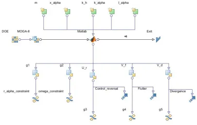
A flow-chart is prepared in order to carry out the optimization work.
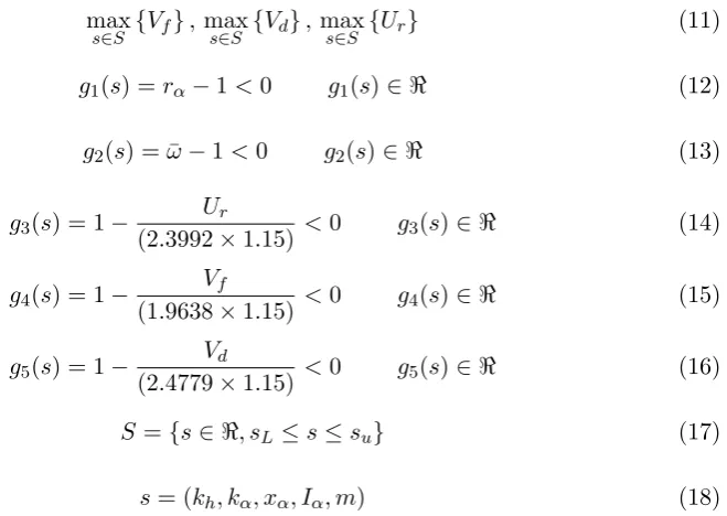
Optimization problem includes 3 objective functions, 5 optimization variables and 5 constraints. The optimization problem can be described as below:
max
s∈S {Vf},maxs∈S {Vd},maxs∈S {Ur} (11)
g1(s) =rα−1<0 g1(s)∈ < (12)
g2(s) = ¯ω−1<0 g2(s)∈ < (13)
g3(s) = 1−
Ur
(2.3992×1.15) <0 g3(s)∈ < (14) g4(s) = 1−
Vf
(1.9638×1.15) <0 g4(s)∈ < (15) g5(s) = 1− Vd
(2.4779×1.15) <0 g5(s)∈ < (16)
S ={s∈ <, sL≤s≤su} (17)
s= (kh, kα, xα, Iα, m) (18)
whereVf,VdandUrdenote the speeds of flutter, divergence and control reversal
instabil-ities respectively whileg1(s),g2(s), g3(s),g4(s), g5(s) are inequality constraints. g1(s),g2(s) indicate the natural constraints for reduced parameters because of physical meaning of the related problem whileg3(s),g4(s), g5(s) require at least 15% increase in instability speeds with respect to the initial design.
sLandsU indicate the lower and upper limits of optimization variables which are stated
in Table 3.
Optimization Variable Lower Limit Upper Limit Reference Study [11]
kh 1.0 r* 5.0 r
-kα 1.0 r 7.0 r
-xα 0.1 0.3 0.2
Iα 1 kgm2 3kgm2 1.2037kgm2
m 7.5kg 12.5 kg 19.258 kg
Table 3. Values of Optimization Variables
* indicates that r is an arbitrary positive real number since the exact value ofkh andkα
can not be determined by using parameters in reference study. These variables are related to natural frequencies. The distinct values of them are not necessarily to be obtained. The lower and upper limits are taken as 1.0 and 5.0 for kh and 1.0 and 7.0 for kα in
optimization process. In order to provide reasonable frequency ratios,g2(s) constraint is defined in the optimization problem.
The optimum designs obtained from the two optimization algorithms are compared in Table 4.
Algorithm Flutter Divergence Control Reversal M OGA−II 3.0436 3.7059 3.2846
N SGA−II 3.0520 3.9272 3.4261 Table 4. Speed Values for Optimum Designs
instabilities with a reasonable mass value between lower and upper limits. Thus, NSGA-II algorithm provides a more effective and faster solution. Optimum design provided by NSGA-II algorithm has design variables defined in Table 5.
kh kα xα Iα m
1.0031 4.1070 0.1000 2.4545kgm2 9.8500 kg Table 5. Design Variables of Optimum Design
The optimum design provides considerable improvement in the speeds of aeroelastic instabilities while still has a less mass with respect to initial design in reference study [11].
4. Flutter Analysis for Three Dimensional Wing Structures
An analytical solution based on assumed mode technique for determination of flutter speed of a three dimensional wing is defined in the present work. Assumed mode technique basically involves the correct representation for replacing displacements with mode shapes and generalized coordinates. Equations of motion can be derived with Lagrange equations including energy equalities and convenient aerodynamic expressions for the flight regime. Flutter boundary is calculated by introducing V-g solution based on artificial damping term.
Displacements of a wing can be determined by product of assumed modes and gener-alized coordinates. Convenient equations for bending and torsional displacements can be obtained in series forms.
w(y, t) =
m
X
i=1
φ(y)·w¯i(t) (19)
θ(y, t) =
n−m
X
i=1
ϕ(y)·θ¯i(t) (20)
where φ and ϕ indicate bending and torsional mode shapes while ¯ω and ¯θ are time dependent generalized coordinates.
Energy equations have to be used to define equations of motion in flutter condition. Firstly, kinetic energy equation can be defined in a general form as:
T = 1 2
l
Z
0
c
Z
0 ˙
w2ρ(x, y)dxdy (21)
In (21),ρ is the density of wing while cshows the chord distance. The equation can be simplified and determined along the spanwise direction.
T = 1 2
l
Z
0
1 2ρdxw˙
2−ρxdxw˙θ˙+1 2x
2ρdxθ˙2
Strain energy equation can also be obtained along the same direction by using the given formula below:
U = 1 2 l Z 0 EI
∂2w¯ ∂y2
2
+GJ
∂2θ¯ ∂y2
2!
dy (23)
where EI and GJ are bending and torsional stiffness values.
Mass, static moment and mass moment of inertia terms vary along the spanwise direc-tion and can be used in flutter equadirec-tions in accordance with their definidirec-tions.
m=ρdy (24) Sy =ρydy (25)
Iy =ρy2dy (26)
Displacements have to be defined according to a reference station, which was placed 3/4 distance of span length from the root of the wing for flutter calculations [10]. In terms of the displacements of reference station (denoted by subscript R) and by using orthogonality, kinetic and strain energy equations can finally be written as below:
T = 1 2w˙
2
R l
Z
0
mφ(y)2dy−wRθR l
Z
0
Syφ(y)ϕ(y)dy+
1 2θ˙
2
R l
Z
0
Iyϕ2(y)dy (27)
U = 1 2ω
2
ωw2R l
Z
0
mφ2(y)dy+1 2ω
2
θθR2 l
Z
0
Iyϕ2(y)dy (28)
In (28), ωω and ωθ indicate the bending and torsional natural frequencies.
Equations of motion can be determined by Lagrange equations and use of free vibration frequencies and energy equalities. In Lagrange equations, generalized forces are related to aerodynamic terms which are lift per unit span and pitching moment about elastic axis.
Qw = `
Z
0
L(y, t)φ(y)dy (29)
Qθ = `
Z
0
My(y, t)ϕ(y)dy (30)
The motion is assumed as harmonic for flutter boundary in order to determine the displacements in reference station.
wR(t) = ˜wReiωt (31)
θR(t) = ˜θReiωt (32)
Aerodynamic loads including sweep angle effects and acting to reference station can be obtained by using Theodorsen aerodynamics [10].
L(y, t) =πρ∞b3ω2cos Λ
wR
b φ(y)Lh−θRϕ(y)
Lα−Lh
1 2+a
(33)
M(y, t) =πρ∞b4ω2cos Λ−wbRφ(y) Mh−Lh 12 +a
+θRπρ∞b4ω2cos Λϕ(y)
h
Mα−(Mh+Lα) 12 +a
+Lh 12 +a
2i
where Λ is sweep angle of the wing. Lh, Lα, Mh, Mα denote the aerodynamic functions of
reduced frequency,k and Theodorsen function, C(k). They can be specified by algebraic functions in terms of reduced frequency for subsonic flow regime where i denotes the complex variable:
Lh = 1−
2i
kC(k) (35) Lα =
1 2−
i k−
2i
kC(k)− 2
k2C(k) (36) Mh=
1
2 (37)
Mα=
3 8 −
i
k (38) Theodorsen function, C(k) can be written in terms of reduced frequency with one pole approach [11]:
C(k) = 1 + 0.4544ik
ik+ 0.1902 (39)
Final equations of motion that lead to the solution of flutter speed are determined after combining the structural and aerodynamic terms by considering taper ratio effect with respect to reference station.
System of equations can finally be written in basic forms as below for flutter solution.
Aw˜R bR
+Bθ˜R= 0 (40)
Cw˜R bR
+Dθ˜R= 0 (41)
whereA, B, C, D are the coefficients of flutter determinant.
Solution of the system includes artificial damping terms to obtain the flutter speed value. Thus, a complex variable, Z, containing these damping effects have to be defined by consideringgw=gθ =g for simplicity.
Z =ωθ ω
2
(1 +ig) (42)
g= 0 is the desired value for the determination of flutter boundary.
Determination of flutter speed for various taper ratio, sweep angle, elasticity and shear modulus values involves the use of both flutter equations and natural frequencies. Thus, flutter equations and natural frequencies have to be expressed in terms of input vari-ables parametrically. Therefore, solution of a flutter problem must include two steps as determination of natural frequencies and calculation of flutter speed.
4.1. Natural Frequency Determination.
System of flutter equations requires use of the first bending and torsional natural fre-quencies. Natural frequencies in bending and torsional motions have to be solved distinctly since the related equations have different physical meanings and mathematical expressions. In free vibration case, the first mode is bending. Therefore, we firstly calculate bending natural frequency.
Equation of motion in bending [13] can be expressed by using an approximate constant value for bending stiffness for simplicity regardless of the wing geometry.
ρA∂ 2w ∂t2 +
∂2 ∂y2 EI∂ 2w ∂y2
where A is effective plate area.
By using separation of variables feature of partial differential equations, we can express the bending displacement term as a product of two functions with single variable.
w(y, t) =M(y)·N(t) (44) whereM(y) andN(t) are position and time dependent functions respectively.
In bending motion, we use 4 boundary conditions in order to calculate the exact value of related natural frequency since the wing structure behaves like a cantilever beam which has clamped and free ends at its root and tip respectively. Thus, we have boundary conditions as: w(0, t) = 0, wy(0, t) = 0, wyy(L, t) = 0 and wyyy(L, t) = 0
Second mode of motion includes torsional displacement. Equation of motion that leads to solution of torsional natural frequency can be specified by the formula given below [13].
∂T ∂y =ρIp
∂2θ
∂t2 (45) where T is torsion andIp is polar moment of inertia.
In a similar way, we can determine torsional natural frequency by using separation of variables approach and boundary conditions in torsional motion as θ(0, t) = 0 and T(L, t) = 0.
5. Validation of Flutter Analysis
The developed flutter analysis procedure is applied to two general wing configurations given by Bisplinghoff [10]. Flutter speeds are determined for these benchmark problems without calculating natural frequencies since the frequencies are already given in the ref-erence. Using these two wings, flutter solutions based on assumed mode technique are performed for validation purposes.
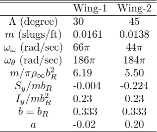
The design parameters for these wing structures are given in Table 6 [10].
Wing-1 Wing-2 Λ (degree) 30 45 m (slugs/ft) 0.0161 0.0138 ωω (rad/sec) 66π 44π
ωθ (rad/sec) 186π 184π
m/πρ∞b2R 6.19 5.50
Sy/mbR -0.004 -0.224
Iy/mb2R 0.23 0.23
b=bR 0.333 0.333
a -0.02 0.20
Table 6. Design Parameters of Benchmark Wings
By using final equations of flutter solution which include taper ratio and sweep angle effects, flutter speeds of each of two models and relative errors with respect to reference solutions are calculated.
6. AGARD 445.6 Flutter Analysis
Reference [10] Calculated Relative Error Wing-1 277 ft/s 279 ft/s 0.8% Wing-2 270 ft/s 268 ft/s 0.7%
Table 7. Flutter Results for Benchmark Problems
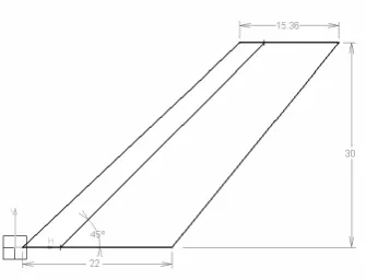
(a) Wing geometry (lengths in inches) (b) The solid model of the wing
Figure 3. AGARD 445.6 Wing Structure [14]
445.6, which is made of laminated mahogany, is a swept-back wing with a sweep angle of 45 degrees, taper and aspect ratios of 0.66 and 1.65 respectively. The airfoil used in this wing is symmetrical NACA65A004 profile. The wing consists of 2 models as solid and weakened models [15]. Wall-mounted weakened model is considered in this work.
Studies in dynamic aeroelastic analysis and flutter calculations of AGARD 445.6 wing are extensive. Several methods have been used to investigate the flutter boundaries. In the work of Beaubien [15], Computational Fluid Dynamics (CFD) is coupled with Com-putational Structural Dynamics (CSD) and time marching simulations are performed by using Euler and Reynolds Averaged Navier Stokes (RANS) equations to calculate flut-ter speed. Lee-Rausch [16] performs linear stability analysis by calculating generalized aerodynamic forces for various values of reduced frequencies. Flutter characteristics are obtained by using V-g analysis which is a similar approach with the present work. Allen [17] shows that the flutter boundaries calculation of AGARD 445.6 with linear methods provides reasonable results since the design and aerodynamics of the wing are simple.
In this work, an analytical flutter analysis for AGARD 445.6 wing is performed by using the determined natural frequencies and flutter equations. Analytical flutter solution methodology which is based on linear techniques is expected to provide good agreement with experiments. In this flutter calculation procedure, the necessary design parameters for reference station of the wing are taken from CAD model constructed in CATIA V5 by Nikbay [14] and also determined from the known geometrical properties of the standart configuration. Material properties of weakened model for natural frequency determination and experimental results for flutter analysis are obtained from the work of Yates [12].
Analytical Experimental [12] Relative Error Bending Frequency (Hz) 9.54 9.60 0.63% Torsional Frequency (Hz) 38.50 38.17 0.86%
Table 8. Natural Frequencies and Relative Errors
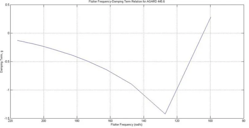
for the realistic wing configuration. Flutter speed of AGARD 445.6 wing is calculated for Mach number of 0.9011 by using analytically determined natural frequency values and then compared to the experimental results stated by Yates [12] and the work of Kolonay [18]. Variation of flutter frequency with respect to artificial damping term,g, is given in Figure 4.
Figure 4. Flutter Frequency-Damping Relation
In Table 9, the results in the works of Yates [12] and Kolonay [18] are included while the relative errors show the differences between the present work and experiment.
Analytical Experimental [12] Kolonay [18] Relative Error ωf (rad/s) 104.25 101.1 99.0 3.12%
Uf (m/s) 308.5 296.7 299.97 3.96%
Table 9. Flutter Results and Relative Errors
Flutter frequency and flutter speed obtained from analytical solution well-agree with the experimental results. Since the analysis for standard configuration results with success, the same procedure can be extended to flutter based aeroelastic optimization with respect to various values of design parameters.
7. Flutter Based Aeroelastic Optimization
elasticity and shear modulus along the spanwise direction of AGARD 445.6 wing. The developed code for the calculation of flutter speed is employed as a tool in deterministic optimization loop while Modefrontier is used as optimization driver.
The objective in this optimization problem is maximizing flutter speed while the opti-mization variables are taper ratio, sweep angle, elasticity and shear modulus of the wing. The optimization problem is defined below:
max
s∈S Uf(s) (46)
S ={s∈ <, sL≤s≤sU}; s= (λ,Λ, Ey, Gy) (47)
0.65< λ <1.0; 0o<Λ<60o; (48) 2000M P a < Ey <3000M P a; 200M P a < Gy <300M P a (49)
where λdenotes taper ratio while Ey and Gy are elasticity and shear modulus values
along spanwise direction.
Broyden-Fletcher-Goldfarb-Shanno (BFGS) is chosen as optimization algorithm with 10 Design of Experiments (DoE).
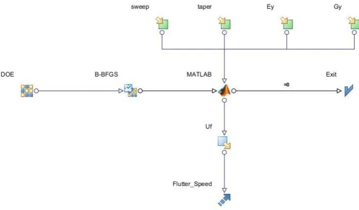
A design with maximum flutter speed of 345.96 m/s is found as optimum among 190 feasible solutions. Design parameters in optimum structure and standard configuration and optimization workflow in Modefrontier can be shown as in Table 10 and Figure 5:
λ Λ (Degree) Ey (MPa) Gy (MPa)
Standard Configuration [12] 0.66 45 3671 409 Optimum Design 0.65 60 2125 287.50
Table 10. Design Parameters of Standard and Optimum Wings
Figure 5. Workflow for Flutter Based Optimization
boundary provides a more reliable flight. Next, the optimum flutter speed and improve-ment with respect to analytical solution are expressed.
Calculated Optimized Flutter Speed (m/s) 308.45 345.96
Improvement ( %) - 12.16
Table 11. Improvement of Flutter Speed in Optimum Design
8. Conclusion
The present study involves improvement of analytical solution techniques for aeroelastic instabilities in two dimensional wing structures and flutter in three dimensional wing models in addition to aeroelastic design optimization for each stated method.
The primary approach is the stability analysis for determination of aeroelastic instabil-ity boundaries such as flutter, divergence and control reversal in two dimensional system. Then the current work is extended to the multi-objective optimization problem to maxi-mize the instability speeds by changing the initial design of the wing model. Two dimen-sional analysis and optimization are preliminary applications for more realistic analysis of three dimensional wing models.
Next, using an analytical flutter solution based on assumed mode technique and aeroe-lastic optimization process to maximize flutter speed are applied to a realistic three dimen-sional wing structure. The analytical solution procedure starts with the use of Lagrange equations. Theodorsen aerodynamics are considered for inviscid, incompressible and sub-sonic flight regime. Additionally, an analytical natural frequency solution is constructed since determination of flutter speed requires the use of bending and torsional natural fre-quencies. The methodology is validated by two benchmark problems from literature and then applied to a realistic wing structure, AGARD 445.6. Firstly, the two free vibration frequencies are determined. Next, flutter speed is obtained for Mach number of 0.9011 in inviscid and incompressible flow. Attaining values for both natural frequencies, flutter frequency and flutter speed are in coherence with the experimental results.
Natural frequencies and flutter speed are solved parametrically with respect to taper ra-tio, sweep angle and material properties of the wing. Therefore, elasticity modulus, shear modulus, taper ratio and sweep angle are selected as optimization variables for flutter based aeroelastic optimization. A Matlab code is developed for autonomous determina-tion of natural frequencies and flutter speed and coupled with the optimizadetermina-tion software Modefrontier. The optimum result provides approximately 12 % of increase in flutter speed.
References
[1] Shubov, M. A., (2004), Mathematical Modeling and Analysis of Flutter in Bending-Torsion Coupled Beams, Rotating Blades and Hard Disk Drives, Journal of Aerospace Engineering, Vol. 17, pp. 256– 269.
[2] Shubov, M. A., (2006), Flutter Phenomenon in Aeroelasticity and Its Mathematical Analysis, Journal of Aerospace Engineering, Vol. 19, No. 1.
[3] Goura, G., (2001), Time Marching Analysis of Flutter Using Computational Fluid Dynamics, (Phd Thesis), University of Glasgow Department of Aerospace Engineering.
[4] Dorf, R. C., Bishop, R. H., (2008), Modern Control Systems, Prentice Hall.
[5] Murty, H. S., (1995), Aeroelastic Stability Analysis of an Airfoil with Structural Nonlinearities Using a State Space Unsteady Aerodynamics Model, AIAA/ASME/ASCE/AHS/ASC Structures, Structural Dynamics, and Materials Conference, New Orleans, USA.
[6] Borglund, R., (2007), Robust Aeroelastic Analysis in the Laplace Domain: Theµ-p Method, Inter-national Forum on Aeroelasticity and Structural Dynamics, Stockholm, Sweden.
[7] Eller, D., (2009), Aeroelasticity and Flight Mechanics: Stability Analysis Using Laplace-Domain Aerodynamics, International Forum on Aeroelasticity and Structural Dynamics, Seattle, USA. [8] Lee, B. H. K., (1984), A Study of Transonic Flutter of a Two-Dimensional Airfoil Using the U-g and
p-k Methods, Canada National Research Council Aeronautical Report.
[9] Ju, Q. and Qin, S., (2009), New Improved g Method for Flutter Solution, Journal of Aircraft, Vol. 46, No. 6, pp. 1284-1286.
[10] Bisplinghoff, R. L., Ashley, H. and Halfman, R. L., (1955), Aeroelasticity, Addison-Wesley Publishing Company.
[11] Dowell, E. H., Crawley, E. F., Curtiss Jr., H. C., Peters, D. A., Scanlan, R. H. and Sisto, F., (1995), A Modern Course in Aeroelasticity, Kluwer Academic Publishers.
[12] Yates, E., (1985), Standard Aeroelastic Configurations for Dynamic Response I-Wing 445.6, AGARD Report No.765.
[13] Scanlan, R. H. and Rosenbaum, R., (1951), Introduction to the Study of Aircraft Vibration and Flutter, The Macmillan Company.
[14] Nikbay, M., Fakkusoglu, N. and Kuru, M. N., (2010), Reliability Based Multi-disciplinary Optimiza-tion of Aeroelastic Systems with Structural and Aerodynamic Uncertainties, 13th AIAA/ISSMO Multidisciplinary Analysis and Optimization (MAO) Conference, Fort Worth, Texas, USA.
[15] Beaubien, R. J., Nitzsche, F. and Feszty, D., (2005), Time and Frequency Domain Flutter Solu-tions for the AGARD 445.6 Wing, International Forum on Aeroelasticity and Structural Dynamics, Munich, Germany.
[16] Lee-Rausch, E. M. and Batina, J. T., (1993), Calculation of AGARD Wing 445.6 Flutter Using Navier-Stokes Aerodynamics, AIAA 11th Applied Aerodynamics Conference, Monterey, California. [17] Allen, C. B., Jones, D., Taylor, N. V., Badcock, K. J., Woodgate, M. A., Rampurawala, A. M., Cooper, J. E. and Vio, G. A., (2004), A Comparison of Linear and Non-Linear Flutter Prediction Methods: A Summary of PUMA DARP Aeroelastic Results, Royal Aeronautical Society Aerody-namics Conference, London.
Melike Nikbaywas born in 1973 in Istanbul. She got her BS degree in 1996 and her MS degree in 1998 both in Mechanical Engineering from Bogazici University. She worked as a Research Engineer at Arcelik R & D Depart-ment between 1996-1998. She got her second MS degree in 1999 and her PhD degree in 2002 in Aerospace Engineering from University of Colorado at Boul-der. She worked as Research Assistant at Center for Aerospace Structures between 1998-2002 in Boulder. She worked as R & D Leader at Kalekalip Defense and Aerospace Division between 2003-2004. She joined ITU in 2004 as assistant professor and has been associate professor in 2011. Her current research interests are multidisciplinary analysis and optimization, aeroelas-ticity and design under uncertainty.