Copyright © The Author(s).All Rights Reserved. Published by American Research Institute for Policy Development DOI: 10.15640/arms.v6n1a2 URL: https://doi.org/10.15640/arms.v6n1a2
Logarithmic Mean and the Difference Calculus
Shu Tsuchida
1Abstract
A logarithmic mean (log-mean) has very useful properties and has been applied over a broad range of fields. Nevertheless, there are more interesting and important areas to solve using this log-mean. The main discussions revolve around two areas. One is the decomposition of a difference or ratio of a function between two periods into two forms: an additive decomposition (AD) and a multiplicative decomposition (MD). To derive an AD and/or an MD for the function; our method (difference calculus) employs a log-mean. Using this method, we derive the ADs and MDs for many functions and compare some results with those derived by the finite-difference calculus (conventional calculus) and the differential calculus. The other area of focus is to show the close correspondences between a difference quotient derived by the difference calculus and a differential quotient, generally called a derivative. From these discussions, we demonstrate three points: our difference calculus has many advantages over the conventional one, some of the results obtained by our calculus can/cannot be used as discrete approximations to those obtained by the differential calculus, and some expressions produced by the difference quotients can/cannot be used as discrete approximations to the differential equations.
Keywords: decomposition, difference calculus, differential calculus, differential equation, discrete approximation, logarithmic mean.
1. Introduction
A logarithmic mean (hereafter log-mean) has very useful properties and has been applied over a broad range of fields [1, 3–6, 10 (see also footnotes 1 and 2 in it), 13, 20–24]. Nevertheless, there are more interesting and important areas to solve using this log-mean. For examples, it can be used to define the hyperbolic function. Moreover, whenever we employ the log-mean to decompose a function, we can easily derive two forms that are similar to those derived by the differential calculus, as we shall show later. We call this new method of derivation the “difference calculus.”2 The results derived by our calculus may produce discrete approximations to those by the differential calculus.
In most of our discussions, most variables are assumed to be economic data, so that they are positive3 and discrete unless events that assume differentiability for their description are considered. (When we discuss these latter events, all variables are assumed to be continuous and differentiable.) In addition, for simplicity, they are usually not unity when we need to take their logarithms and only the natural logarithm is used.
Consider any two positive variables, x0 and x1, where the subscript 0 represents a base period and 1 a comparison period. Their difference is written as Δx10 = x1 – x0, and the logarithmic difference as Δlogx10 = logx1 – logx0 = log(x1/x0). For differentials, that is, under an infinitesimal change, they are naturally written as dx and dlogx. For finite changes, the two differences above, which include those of dependent and independent variables for some
1Independent Marketing Consultant: 7-521, 2913, Nara-Cho, Aoba-Ku, Yokohama City, Kanagawa 227-0036, Japan
2Some points discussed below are explained in [19].
functions, are also assumed to be non-zero so as to obtain an interesting result. A log-mean is defined by
𝐿(𝑥) ≡ ∆𝑥10
∆ log 𝑥10=
𝑥1− 𝑥0 log 𝑥1− log 𝑥0=
𝑥1− 𝑥0 log(𝑥1⁄ )𝑥0 =
𝑥0− 𝑥1
log(𝑥0⁄ )𝑥1 . (1)
For clarity of expression, we write the log-mean (1) as L(x) to explain its basic properties and applications in the two sections below. To explain further useful properties, we need to write the two arguments for the log-mean explicitly. Hence, we write the log-mean (1) as L(x1, x0), as in Section 4. Our data are discrete, i.e., not continuous, so the integral representations of the log-mean, which may be interesting (see, for example, [8, 16, 18]), are discarded.
The remainder of this paper is organized as follows. In Section 2, we briefly explain basic properties of the log-mean. Other properties of the log-mean, which includes the relationship between this mean and the usual three means (arithmetic, geometric, and harmonic) as well as the connection between this mean and hyperbolic functions, are explained in Section 4. In Section 3, we show its applications to two areas. First, we show decompositions for some functions using two forms: an additive form and a multiplicative form. Therein, the results derived by our difference calculus that may employ the log-mean are compared with those by the conventional difference calculus (or finite-difference calculus, hereafter “conventional calculus”) and the differential calculus. Second, we define a difference quotient that commonly makes the most of some log-means and show its close relationship to the differential quotient. (Remember that a form with a dependent variable given by the latter is usually called the differential equation as will be shown later.) All these aspects will make it clear that our difference calculus has many advantages over the conventional calculus, and some of the results produced by our difference calculus and quotient can be used as discrete approximations to those by the differential calculus and equation. Since a log-mean is defined for only positive variables, the scope of our difference calculus is somewhat restricted. To broaden the scope, we shall in Appendix A explain a method for handling non-positive variables; the remarks are conjectural as it has a few drawbacks. Conclusions are given in Section 5.
2. Basic Properties of a Logarithmic Mean
We briefly explain some basic properties of the log-mean (for its basic properties, see also [4–6, 8, 13, 20, 21, 23]). This value is always positive and has the limit:
lim
∆𝑥10→0𝐿(𝑥) = 𝑥1 = 𝑥0. (2)
This limit induces correspondence between the difference and differential calculi to be shown later. If 𝑥1⁄𝑥0 is close to 1, it can be approximated by the three usual means: arithmetic, geometric, and harmonic (see Subsection 4.1). This property plays an important role, when we compare the results derived by the difference and conventional calculi (see below).
Other useful properties are
∑ 𝐿(𝑥𝑖)
𝑖 ⁄𝐿 (∑ 𝑥𝑗 𝑗)≤ 1, (3)
𝐿(𝑥2) =(𝑥1)2− (𝑥0)2 2(Δlog 𝑥10) =
(𝑥1+ 𝑥0)(𝑥1− 𝑥0)
2(Δlog 𝑥10) = 𝐴(𝑥)𝐿(𝑥), (4)
∑ 𝐿(𝑤𝑖)
𝑖 Δlog(𝑤𝑖10) = ∑ ∆𝑤𝑖 𝑖10= ∑ (𝑤𝑖 𝑖1− 𝑤𝑖0)= 0, (5)
where A(x) = (x1+ x0)/2 is the arithmetic mean;4 and wit = xit/(∑ 𝑥𝑗 𝑗𝑡), the subscript t (t = 0, 1, …) represents a period, i (or j) the ith (or jth) commodity, and the summation is made over all commodities. Eq. (4) is often used in our difference calculus below.
When a positive x approaches zero, we have the approximation that is called the log-approximation in this paper: log 𝑥 ≈ x − 1. This approximation yields 𝐿(𝑥) ≈ 𝑥0≈ 𝑥1, because
𝐿(𝑥) =𝑥0(𝑥1⁄𝑥0− 1)
∆ log 𝑥10 =
𝑥1(𝑥0⁄𝑥1− 1)
∆ log 𝑥01 ,
wherein ∆ log 𝑥10= log(𝑥1⁄ ) = − log(𝑥𝑥0 0⁄ )𝑥1 . See also Subsection 4.2. 3. Applications
3.1. Additive and Multiplicative Decompositions
We present the difference or ratio of a function between two periods using two forms: an additive form of which all components are additive differences and a multiplicative form of which all components are logarithmic differences. We call the former an additive decomposition (AD) and the latter a multiplicative decomposition (MD). To derive an AD and an MD for some functions, we may employ three methods: the conventional, difference, and differential calculi. One may notice that the AD and MD derived by the first two calculi may relate to those derived by the last. We explain these in this order. (There are a few functions to which the first two methods cannot be applied.) While the conventional and differential calculi are well-known, the difference calculus (i.e., our method) is less-known. Hence, we shall present many examples illustrating by our method (see also Subsection 3.2 and Appendixes A and B).
Comparing the conventional and difference calculi, we find that the former can give an AD and/or an MD for only a few functions, and the latter can apply to many functions (see also Appendix B). We would like to emphasize that the difference calculus needs to employ a log-mean to derive an AD and/or an MD.
3.1.1. Conventional Calculus
This method relates to that called the “calculus of finite differences” [75, 176]. Most differences of independent variables for a function used by the latter are unity, as in [7], which implies ΔX10 = X1 – X0 = (X+1) – X = 1. Jordan [14], however, uses the following difference: ∆𝑋𝑡+1,𝑡= 𝑋𝑡+1− 𝑋𝑡= ℎ, in which h is independent of t
and always constant. While the conventional calculus can quickly derive an MD for any multiplicative function, it can derive an AD for only those functions composed of two independent variables as shown in Examples 1* and 2* below. (For other functions, see our extended method given in Appendix B). In contrast, this method can easily derive an AD for any additive function, but it cannot derive an MD for that as shown in Example 3* below. These derivations are also explained in the relevant text books (for example, [12, 17]).
1) Example 1*: Yt =XtZt.7
The MD of this multiplicative function is easily obtained as follows: ∆ log 𝑌10= ∆ log 𝑋10+ ∆ log 𝑍10. Each term on the right-hand side is X’s or Z’s contribution to ΔlogY10.
The AD of this is
𝑌1− 𝑌0 = 𝑋1𝑍1− 𝑋0𝑍1+ 𝑋0𝑍1− 𝑋0𝑍0= 𝑋1𝑍1− 𝑋1𝑍0+ 𝑋1𝑍0− 𝑋0𝑍0. ∴ ∆𝑌10= 𝑍1∆𝑋10+ 𝑋0∆𝑍10or ∆𝑌10 = 𝑍0∆𝑋10+ 𝑋1∆𝑍10. (6)
Each term on the right-hand sides in Eq. (6) is X’s or Z’s contribution to ΔY10. Whereas a convex combination of the two equations in Eq. (6) is also the AD, the arithmetic mean of those is often used as the AD, specifically
∆𝑌10= 𝐴(𝑍)∆𝑋10+ 𝐴(𝑋)∆𝑍10. (7)
For multiple multiplicative functions, such as Yt =WtXtZt, we are able to derive the AD for such functions using the more awkward procedures (see Appendix B for details).
2) Example 2*: Yt =Xt/Zt, (𝑋𝑡 ≠ 𝑍𝑡).
5Boole [7] was the first to present this subject from the modern viewpoints. See Jordan [14, footnote 1 and Carver’s introduction
in it]. This is also called the “finite-difference calculus” (see online [11]).
Because the MD is easily obtained, we omit it here. The AD is
∆𝑌10 =
𝑋1
𝑍1−
𝑋0
𝑍0=
𝑋1𝑍0− 𝑋0𝑍0+ 𝑋0𝑍0− 𝑋0𝑍1
𝑍1𝑍0 =
𝑍0∆𝑋10− 𝑋0∆𝑍10 𝑍1𝑍0
Comparing this decomposition with Eq. (6), we see that we have another AD. From its arithmetic mean, an AD similar to Eq. (7) is obtained:
∆𝑌10=𝐴(𝑍)∆𝑋10− 𝐴(𝑋)∆𝑍10
𝑍1𝑍0 (8)
To obtain the AD of functions such as Yt =Wt/XtZt, we need to use the more awkward procedures presented in Appendix B.
3) Example 3*: Yt =Xt + Zt.
Since the AD for this additive function is quickly obtained, it is omitted. The MD of this is not obtained. 4) Example 7*: 𝑌𝑡 = (𝑋𝑡)𝐶𝑡.
The conventional method can give neither an AD nor an MD for this function.
3.1.2. Difference Calculus
The difference calculus is easily able to yield ADs and MDs for many functions. Some of our methods below can be found in [5, e.g., pp. 126–132]. See also [1, 9]. Our scope is, however, wider than these.
1) Example 1: Yt =XtZt.
Taking the logarithm of both sides produces the MD:
∆ log 𝑌10= ∆ log 𝑋10+ ∆ log 𝑍10. As ∆𝑥10= 𝐿(𝑥)∆ log 𝑥10, we quickly obtain its AD given by
∆𝑌10= (𝐿(𝑌) 𝐿(𝑋)⁄ )∆𝑋10+ (𝐿(𝑌) 𝐿(𝑍)⁄ )∆𝑍10. (9)
If we apply the log-approximation to three log-means in Eq. (9), we have two ADs in Eq. (6).8 In addition, using the approximation L(x) ≈G(x) ≈A(x) (see Subsection 4.1 for details), we find that Eq. (7) can be approximated by Eq. (9) (see also Appendix B).
Even if one of the independent variables is non-positive, our method may be able to derive only its AD (see Appendix A). Our approach can easily decompose more complex functions such as Yt =XtZtWt and Yt=(Xt)2(ZtWt); see examples below and Appendix B.
2) Example 2: Yt =Xt/Zt, (Xt≠Zt.).
The difference calculus quickly produces the following MD and AD: ∆ log 𝑌10= ∆ log 𝑋10− ∆ log 𝑍10,
∆𝑌10= (𝐿(𝑌) 𝐿(𝑋)⁄ )∆𝑋10− (𝐿(𝑌) 𝐿(𝑍)⁄ )∆𝑍10. (10)
Using the approximation above, we also find that Eq. (8) can be approximated by Eq. (10).
Comparing Example 1 with Example 2, Eq. (9) with Eq. (7), and Eq. (10) with Eq. (8), we see that our calculus yields more elegant forms than those derived by the conventional calculus. For the multiplicative functions composed of three or more independent variables, see Appendix B.
3) Example 3: Yt =Xt + Zt. The AD is
∆𝑌10 = ∆𝑋10+ ∆𝑍10, from which, we can derive the following MD:
∆ log 𝑌10 = (𝐿(𝑋) 𝐿(𝑌)⁄ )∆ log 𝑋10+ (𝐿(𝑍) 𝐿(𝑌)⁄ )∆ log 𝑍10. Note that the conventional calculus cannot derive this MD.
4) Example 4: Yt =Xt + WtZt.
Letting Vt = WtZt, we deduce its AD and MD using Example 1. ∆ log 𝑉10= ∆ log 𝑊10+ ∆ log 𝑍10.
∆𝑉10= (𝐿(𝑉) 𝐿(𝑊)⁄ )∆𝑊10+ (𝐿(𝑉) 𝐿(𝑍)⁄ )∆𝑍10.
Using the latter equation, we produce
∆𝑌10= ∆𝑋10+ (𝐿(𝑉) 𝐿(𝑊)⁄ )∆𝑊10+ (𝐿(𝑉) 𝐿(𝑍)⁄ )∆𝑍10.
∆ log 𝑌10= (𝐿(𝑋) 𝐿(𝑌)⁄ )∆ log 𝑋10+ (𝐿(𝑉) 𝐿(𝑌)⁄ )(∆ log 𝑊10+ ∆ log 𝑍10).
The conventional calculus cannot derive either AD or MD. For the examples below, the same can also be stated. 5) Example 5: Yt = exp(Xt).
The MD and AD are
∆ log 𝑌10= 𝐿(𝑋)∆ log 𝑋10,
∆𝑌10= 𝐿(𝑌)∆𝑋10.
6) Example 6: Ht = ptlog(1/pt) =–ptlogpt> 0 and 0 < pt< 1.
This function is frequently used in information theory. Here, we can employ two methods. Using qt = 1/pt> 1, we directly decompose this function (Case 1 below) and then decompose this by another method (Case 2 below). As their ADs are easily obtained from the corresponding MD, we omit the details. The two derived MDs are naturally the same.
Case 1: Ht = ptlogqt.
Taking the logarithm of both sides yields the following, from which we can derive its MD. Note that logqt is always positive.
log 𝐻𝑡 = log 𝑝𝑡+ log(log 𝑞𝑡), ∴ ∆ log 𝐻10= ∆ log 𝑝10+∆ log 𝑞10
𝐿(log 𝑞)= ∆ log 𝑝10−
∆ log 𝑝10
𝐿(log 𝑞) = ∆ log 𝑝10(1 −
1 𝐿(log 𝑞)) , wherein ∆ log 𝑞10= −∆ log 𝑝10and 𝐿(log 𝑞) is defined by
𝐿(log 𝑞) = log 𝑞1− log 𝑞0
log(log 𝑞1) − log(log 𝑞0)=
∆ log 𝑞10 ∆ log log 𝑞10 , wherein
∆ log log 𝑞10≡ log(log 𝑞1) − log(log 𝑞0). Case 2: Ht = –ptlogpt.
Squaring both sides and taking their logarithms, we have 2log 𝐻𝑡= 2 log 𝑝𝑡+ logΨ𝑡, where Ψ𝑡 = (log 𝑝𝑡)2. From this equation, we obtain
∆ log 𝐻10= ∆ log 𝑝10+ ∆Ψ10
2𝐿(Ψ)=Δlog 𝑝10+
𝐴(log 𝑝)Δlog 𝑝10
𝐿(Ψ) ,
where
𝐿(Ψ) =ΔΨ10⁄ΔlogΨ10,
∆Ψ10= (log 𝑝1+ log 𝑝0)(log 𝑝1− log 𝑝0) = 2𝐴(log 𝑝)Δlog 𝑝10, 𝐿(Ψ) = 𝐿((log 𝑝)2) = 𝐿((log 𝑞)2) = 𝐴(log 𝑞)𝐿(log 𝑞) = −𝐴(log 𝑝)𝐿(log 𝑞) Recall that A(log 𝑞) = −𝐴(log 𝑝) > 0 and 𝐿(log 𝑝) cannot be defined. Thus,
∆ log 𝐻10= ∆ log 𝑝10−
∆ log 𝑝10
𝐿(log 𝑞) = ∆ log 𝑝10(1 −
1 𝐿(log 𝑞)). 7) Example 7: 𝑌𝑡 = (𝑋𝑡)𝐶𝑡.
We show only two MDs obtained under two local (i.e., non-global) assumptions that exclude events such as
𝐴(log 𝑋) = 0 and 𝐴(log 𝑌) = 0. (For cases including these events, see Appendix A.) Taking the logarithm of both
sides leads to
log 𝑌𝑡 = 𝐶𝑡log 𝑋𝑡. (11)
Assumption1: Xt < 1.
where
Φ𝑡 = (log 𝑌𝑡)2,ΔΦ10= (log 𝑌1+ log 𝑌0)(log 𝑌1− log 𝑌0) = 2𝐴(log 𝑌)Δlog 𝑌10, Γ𝑡 = (𝐶𝑡)2,ΔΓ10= 2𝐴(𝐶)Δ𝐶10= 2𝐴(𝐶)𝐿(𝐶)∆ log 𝐶10,
Ψ𝑡 = (log 𝑋𝑡)2,ΔΨ10= 2𝐴(log 𝑋)Δlog 𝑋10.
Note that three arithmetic means are nonzero. From these and the three log-means
𝐿(Φ) =ΔΦ10⁄ΔlogΦ10, 𝐿(Γ) =ΔΓ10⁄ΔlogΓ10 = 𝐿(𝐶2) = 𝐴(𝐶)𝐿(𝐶), and 𝐿(Ψ) =ΔΨ10⁄ΔlogΨ10,
we derive the MD:
ΔΦ10
𝐿(Φ) =
ΔΓ10 𝐿(Γ)+
ΔΨ10 𝐿(Ψ),
∴ ∆log 𝑌10= 𝐿(Φ)
𝐴(log 𝑌){∆ log 𝐶10+
𝐴(log 𝑋)
𝐿(Ψ) ∆ log 𝑋10}. (12)
Assumption 2: Xt> 1.
Because logXt> 0 and logYt> 0, we can further take the logarithm of both sides of Eq. (11) and obtain the MD:
Δlog log 𝑌10=Δlog 𝐶10+Δlog log 𝑋10,
∴ ∆ log 𝑌10 = 𝐿(log 𝑌)∆ log 𝐶10+
𝐿(log 𝑌)
𝐿(log 𝑋)∆ log 𝑋10, (13)
where L(logY) and L(logX) are defined in a similar way to the above. In this case, we obtain 𝐿(Φ) = 𝐴(log 𝑌)𝐿(log 𝑌)and 𝐿(Ψ) = 𝐴(log 𝑋)𝐿(log 𝑋). Thus, we may also use Eq. (12), because Eq. (12) degenerates in to Eq. (13) under Assumption 2.
3.1.3. Differential Calculus
Our difference calculus is closely related to the differential calculus. The log-mean yields
∆ log 𝑥10= ∆𝑥10⁄𝐿(𝑥). (14)
By contrast, the differential calculus produces
d log 𝑥 = d𝑥 𝑥⁄ . (15)
Comparing Eq. (14) with Eq. (15), we establish correspondences (a finite-change variable ↔ an infinitesimal-changevariable),
∆ log 𝑥10↔ d log 𝑥, ∆𝑥10 ↔ d𝑥, and 𝐿(𝑥) ↔ 𝑥.
The last correspondence follows from Eq. (2).
We show the ADs and MDs for some functions using the differential calculus. These may or may not induce the correspondences above. Wherever these correspondences are found, the AD or MD derived by the difference calculus can be used as the discrete approximation to that obtained by the differential calculus.
1) Example 1**: Y = XZ.9
d𝑌 = 𝑍d𝑋 + 𝑋d𝑍. dlog 𝑌 = d log 𝑋 + d log 𝑍. Thus, 𝐿(𝑌) 𝐿(𝑋)⁄ ↔ 𝑌 𝑋⁄ = 𝑍 and𝐿(𝑌) 𝐿(𝑍)⁄ ↔ 𝑌 𝑍⁄ = 𝑋.
2) Example 4**: Y = X + WZ.
d𝑌 = d𝑋 + 𝑍d𝑊 + 𝑊d𝑍.
𝑌d log 𝑌 = 𝑋d log 𝑋 + 𝑊𝑍d log 𝑊 + 𝑊𝑍d log 𝑍,
∴ d log 𝑌 = (𝑋 𝑌⁄ )d log 𝑋 + (𝑊𝑍 𝑌⁄ )(d log 𝑊 + d log 𝑍).
The above-stated correspondences are evident. 3) Example 5**:Y = exp(X)
d𝑌 =exp(𝑋)d𝑋 = 𝑌d𝑋. d log 𝑌 = 𝑋d log 𝑋. Again, the foregoing correspondences are evident.
4) Example 7**: 𝑌 = 𝑋𝐶. We show only the MD,
d log 𝑌 = log 𝑋 d𝐶 + 𝐶d log 𝑋 = (𝐶 log 𝑋) d log 𝐶 + 𝐶d log 𝑋,
which holds for any positive X. Hence, the MD does not necessarily have the correspondences stated above, which does only if X > 1 (compare the above with Eq. (12) and Eq. (13)).
3.2. Difference Calculus for a Complex Function
There is a complex function having an additive-multiplicative term such as (x+w)/z or (z – w)2 = (z – w)(z –
w). To apply our difference calculus to this function, we may need to transform the variables. If such transformation of variables must be considered, the difference calculus may have multivalent ADs and MDs. On the contrary, the differential calculus always produces a univalent AD and MD. Our multivalent ADs and MDs, however, produce the same values as these univalent AD and MD, if all the changes in variables approach zero. To simplify the discussion in what follows, we show some examples using only ADs without the subscript t.
1) Example 8: Y = X(Z – W) = XF = G – H.
Here, F = Z – W, G =XZ, and H = XW. The differential calculus leads to the AD given by d𝑌 = (𝑍 − 𝑊)d𝑋 + 𝑋d𝑍 − 𝑋d𝑊.
Recalling our assumptions (i.e., Y, X, Z, and W are positive; so F > 0), the difference calculus provides two ADs. 1) With F = Z – W, the AD is obtained from
∆ log 𝑌 = ∆ log 𝑋 + ∆ log 𝐹 , ∆𝐹 = ∆𝑍 − ∆𝑊.
∴ ∆𝑌 =𝐿(𝑌)
𝐿(𝑋)∆𝑋 +
𝐿(𝑌)
𝐿(𝐹)∆𝐹 =
𝐿(𝑌)
𝐿(𝑋)∆𝑋 +
𝐿(𝑌)
𝐿(𝐹)∆𝑍 −
𝐿(𝑌)
𝐿(𝐹)∆𝑊. (16)
2) With G = XZ and H = XW, the AD follows from equations:
∆𝑌 = ∆𝐺 − ∆𝐻, ∆ log 𝐺 = ∆ log 𝑋 + ∆ log 𝑍 , ∆ log 𝐻 = ∆ log 𝑋 + ∆ log 𝑊,
∴ ∆𝑌 = (𝐿(𝐺)
𝐿(𝑋)−
𝐿(𝐻)
𝐿(𝑋)) ∆𝑋 +
𝐿(𝐺)
𝐿(𝑍)∆𝑍 −
𝐿(𝐻)
𝐿(𝑊)∆𝑊. (17)
These separate contributions to ΔY from X, Z, and W in Eq. (16) and Eq. (17) are different. The question now arises: which set of contributions should be selected as the best. We want to leave the matter open. (In the example below, a similar problem arises.)
If, however, the changes in each variable approach zero, each contribution approaches the differential results:
𝐿(𝑌)
𝐿(𝑋)↔ 𝑍 − 𝑊,
𝐿(𝐺)
𝐿(𝑋)−
𝐿(𝐻)
𝐿(𝑋)↔ 𝑍 − 𝑊,
𝐿(𝑌)
𝐿(𝐹)↔ 𝑋,
𝐿(𝐺)
𝐿(𝑍)↔ 𝑋,
𝐿(𝐻)
𝐿(𝑊)↔ 𝑋.
This property also holds in the example below.
2) Example 9 (saving ratio): b = (Y – C)/Y = S/Y= 1– a.
Here, S = Y – C and a = C/Y; and the quantities Y, C, S, a, and b are, respectively, income, consumption, saving, propensity to consume, and saving ratio. For dissaving (i.e., S < 0 and b < 0), see the discussion in Appendix A. The differential calculus yields:
d𝑏 =𝐶d𝑌
𝑌2 −
d𝐶 𝑌. The difference calculus yields two ADs.
1) For b = S/Y,
∆ log 𝑏 = ∆ log 𝑆 − ∆ log 𝑌 , ∆𝑆 = ∆𝑌 − ∆𝐶,
∴ ∆𝑏 = (𝐿(𝑏)𝐿(𝑆)−𝐿(𝑏)
𝐿(𝑌)) ∆𝑌 −
𝐿(𝑏)
𝐿(𝑆)∆𝐶.
2) For b =1– a,
∴ ∆𝑏 =𝐿(𝑎)
𝐿(𝑌)∆𝑌 −
𝐿(𝑎)
𝐿(𝐶)∆𝐶.
3.3. Difference Quotient versus Differential Quotient
As dY/dX is sometimes called the differential quotient, we call ΔY/ΔX a “difference quotient.” We recall the natural fundamental definition of the differential quotient:
lim ∆𝑋→0
∆𝑌
∆𝑋≡
d𝑌 d𝑋.
The result derived by the differential quotient, which will be explained below, is the differential equation. Thus, that derived by the difference quotient is regarded as the discrete approximation to this equation from the definition above. Considering the correspondences shown in Subsubsection 3.1.3, we are able to find a situation wherein the difference quotient corresponds to the differential one. Inspired by Subsection 3.2, we come to the understanding that not all functions can yield the difference quotients that directly correspond to their differential versions. Moreover, our method of deriving difference quotients does not apply to some functions such as trigonometric functions, because the arguments for the log-mean must be positive. We now discuss some examples. In the following, we omit the subscripts t on all functions and their difference forms to stress these correspondences.
1) Y= (X)n, where n is a non-zero constant.10
∆ log 𝑌 = ∆𝑌 𝐿(𝑌)⁄ = 𝑛∆ log 𝑋 = 𝑛(∆𝑋 𝐿(𝑋)⁄ ).
Thus, the difference quotient is
∆𝑌
∆𝑋= 𝑛
𝐿(𝑌) 𝐿(𝑋) .
In contrast, we have the following differential quotient, the form of which is typical of a differential equation, d𝑌
d𝑋= 𝑛𝑋𝑛−1= 𝑛
𝑋𝑛
𝑋 = 𝑛
𝑌 𝑋 .
Provided that ΔX approaches 0, as in the definition above, the difference and differential quotients are close. Besides, replacing L(z) with z, we can obtain the right hand of the latter from that of the former. Thus, the result produced by the former is also regarded as the discrete approximation to the differential equation. (The same property holds in the examples below.)
2) Y = exp(X).
Example 5 and Example 5** in Subsection 3.1 produce ∆𝑌
∆𝑋= 𝐿(𝑌) and
d𝑌
d𝑋=exp(𝑋) = 𝑌. 3) Y= 𝒂𝑿, 𝑎 > 0 is constant.
∆ log 𝑌 = ∆𝑋(log 𝑎),∆𝑌
∆𝑋= 𝐿(𝑌) log 𝑎 , and
d𝑌
d𝑋= 𝑌 log 𝑎.
Compare our difference quotient with Boole’s [7, p. 10].11
4) Y = FG, where F= (X)2 + a > 0, G= X + b > 0; and a and b are constants. ∆ log 𝑌 = ∆ log 𝐹 + ∆ log 𝐺,
∆𝑌 = (𝐿(𝑌) 𝐿(𝐹)⁄ )∆𝐹 + (𝐿(𝑌) 𝐿(𝐺)⁄ )∆𝐺. (18)
Setting C = (X)2, we have ∆ log 𝐶 = 2∆ log 𝑋. Hence,
∆𝐹 = ∆𝐶 = 2(𝐿(𝐶) 𝐿(𝑋)⁄ )∆𝑋. (19)
Substituting Eq. (19) and ΔG = ΔX into Eq. (18) yields
∆𝑌 = 2(𝐿(𝑌) 𝐿(𝐹)⁄ )(𝐿(𝐶) 𝐿(𝑋)⁄ )∆𝑋 + (𝐿(𝑌) 𝐿(𝐺)⁄ )∆𝑋,
∴ ∆𝑌
∆𝑋=
2𝐿(𝑌)𝐿(𝑋2)
𝐿(𝐹)𝐿(𝑋) +
𝐿(𝑌) 𝐿(𝐺) .
In contrast, the differential quotient is
d𝑌 = 𝐺d𝐹 + 𝐹d𝐺 = 2𝐺𝑋d𝑋 + 𝐹d𝑋,
∴d𝑌
d𝑋= 2𝐺𝑋 + 𝐹 =
2𝑌𝑋2
𝐹𝑋 +
𝑌 𝐺 .
4. Further Properties of the Logarithmic Mean
4.1. Comparison of the Logarithmic Mean with the Usual Three Means
In this section, we explicitly write the two arguments for the logarithmic, arithmetic, geometric, and harmonic means, specifically, L(x1, x0), A(x1, x0), G(x1, x0), and H(x1, x0) for two positive variables, x1 and x0. These are also rewritten as x0L(x1/x0, 1), x0A(x1/x0, 1), x0G(x1/x0, 1), and x0H(x1/x0, 1). Hence, we have A(x1, x0)/L(x1, x0) =A(x1/x0, 1)/L(x1/x0, 1), G(x1, x0)/L(x1, x0) = G(x1/x0, 1)/L(x1/x0, 1), etc.12 For a positive constant c, all the means have the following properties:
𝐿(𝑐𝑥1, 𝑐𝑥0) =
𝑐𝑥1− 𝑐𝑥0
log(𝑥1⁄ )𝑥0 =
𝑐(𝑥1− 𝑥0)
log(𝑥1⁄ )𝑥0 = 𝑐𝐿(𝑥1, 𝑥0), 𝐴(𝑐𝑥1, 𝑐𝑥0) = 𝑐𝐴(𝑥1, 𝑥0), 𝐺(𝑐𝑥1, 𝑐𝑥0) = 𝑐𝐺(𝑥1, 𝑥0), and 𝐻(𝑐𝑥1, 𝑐𝑥0) = 𝑐𝐻(𝑥1, 𝑥0).
When the absolute value w is very small13, we obtain
𝐿(1 + 𝑤, 1) = 𝑤
log(1 + 𝑤)≈ 1 (1 −
1
2𝑤 +
1 3𝑤2)
⁄ ,
wherein we used log(1 + 𝑤) ≈ 𝑤 − (1 2⁄ )𝑤2+ (1 3⁄ ) 𝑤3, and
𝐺(1 + 𝑤, 1) = (1 + 𝑤)0.5≈ 1 +1
2𝑤 −
1 8𝑤2. By contrast, the arithmetic mean is
𝐴(1 + 𝑤, 1) = 1 +𝑤
2 . Hence, we find
𝐺(1 + 𝑤, 1)
𝐿(1 + 𝑤, 1)≈ 1 −
1 24𝑤2, 𝐴(1 + 𝑤, 1)
𝐿(1 + 𝑤, 1)≈ 1 +
2 24𝑤2. These approximations lead to
𝐺(1 + 𝑤, 1)
𝐴(1 + 𝑤, 1)≈ 1 −
3 24𝑤2, and
2𝐺(1 + 𝑤, 1)
𝐿(1 + 𝑤, 1)+
𝐴(1 + 𝑤, 1)
𝐿(1 + 𝑤, 1)≈ 3,
∴ 𝐿(1 + 𝑤, 1) ≈ (2𝐺(1 + 𝑤, 1) + 𝐴(1 + 𝑤, 1)) 3 .⁄
The last approximation is the same as that given in [8, 15].14 Because the ratio of the harmonic mean to the log-mean is given by
12If x1/x0 = 1, then all four means are equal. 13Since 1+w> 0 is assumed, –1 <w.
14We also find that the Heron mean for p = 1 defined by (G(1 + w, 1) + 2A(1 + w, 1))/3 is greater than or equal to the log-mean
𝐻(1 + 𝑤, 1)
𝐿(1 + 𝑤, 1) = (
𝐺(1 + 𝑤, 1)
𝐿(1 + 𝑤, 1))
2
(𝐿(1 + 𝑤, 1)
𝐴(1 + 𝑤, 1)),
we have the following approximation using the two approximations given above: 𝐻(1 + 𝑤, 1)
𝐿(1 + 𝑤, 1) ≈ 1 −
4 24𝑤2. Therefore, the three approximations lead to
𝐻(1 + 𝑤, 1) ≤ 𝐺(1 + 𝑤, 1) ≤ 𝐿(1 + 𝑤, 1) ≤ 𝐴(1 + 𝑤, 1).
If the absolute value of Δx10/x0 is very small, we can utilize these approximations in the foregoing ratios such as A(x1, x0)/L(x1, x0) because x1/x0 = 1+Δx10/x0. Thus, the log-mean may be approximated by the usual three means. For the actual errors produced by the approximations, see [21, Table 1]. These approximations are handy, when we compare the results derived by the difference and conventional calculi (see Appendix B).
The usual three means have helpful properties given by
𝐴(𝐴(𝑎, 𝑏), 𝐴(𝑐, 𝑑)) = 𝐴(𝐴(𝑎, 𝑐), 𝐴(𝑏, 𝑑)) = 𝐴(𝐴(𝑎, 𝑑), 𝐴(𝑏, 𝑐)) = 𝐴(𝑎, 𝑏, 𝑐, 𝑑), 𝐺(𝐺(𝑎, 𝑏), 𝐺(𝑐, 𝑑)) = 𝐺(𝐺(𝑎, 𝑐), 𝐺(𝑏, 𝑑)) = 𝐺(𝐺(𝑎, 𝑑), 𝐺(𝑏, 𝑐)) = 𝐺(𝑎, 𝑏, 𝑐, 𝑑), 𝐻(𝐻(𝑎, 𝑏), 𝐻(𝑐, 𝑑)) = 𝐻(𝐻(𝑎, 𝑐), 𝐻(𝑏, 𝑑)) = 𝐻(𝐻(𝑎, 𝑑), 𝐻(𝑏, 𝑐)) = 𝐻(𝑎, 𝑏, 𝑐, 𝑑),
where a, b, c, and d are positive variables, A(A(a, b), A(c, d)) is the arithmetic mean for any paring, A(a, b, c, d) is that for four variables, and so on. Conversely, the log-mean does not always retain this property. We present a simple example. Given that a = 1, b = 2, c = 3, and d = 4, we have
𝐿(𝐿(𝑎, 𝑏), 𝐿(𝑐, 𝑑)) = 2.31225 … , 𝐿(𝐿(𝑎, 𝑐), 𝐿(𝑏, 𝑑)) = 2.31221 …, 𝐿(𝐿(𝑎, 𝑑), 𝐿(𝑏, 𝑐)) = 2.31188 ….
∴ 𝐿(𝐿(𝑎, 𝑏), 𝐿(𝑐, 𝑑)) ≠ 𝐿(𝐿(𝑎, 𝑐), 𝐿(𝑏, 𝑑)) ≠ 𝐿(𝐿(𝑎, 𝑑), 𝐿(𝑏, 𝑐)) ≠ 𝐿(𝐿(𝑎, 𝑏), 𝐿(𝑐, 𝑑)).
These pedantic derivations are very difficult, because we must calculate, for example, the following 𝑥 − 𝑦 or 𝑥 𝑦⁄ : 𝐿(𝑎, 𝑏) = 1 log 2, 𝐿⁄ (𝑐, 𝑑) = 1 log(4 3⁄ ⁄ ), and 𝐿(𝐿(𝑎, 𝑏), 𝐿(𝑐, 𝑑)) = 𝑥;
𝐿(𝑎, 𝑐) = 2 log 3, 𝐿⁄ (𝑏, 𝑑) = 2 log 2⁄ , and 𝐿(𝐿(𝑎, 𝑐), 𝐿(𝑏, 𝑑)) = 𝑦.
Note that these logarithms are transcendental (i.e., irrational) numbers. From these inequalities and the results shown in Section 3 and Subsection 4.3 below, we infer that the log-means for three or more variables (e.g., those defined by [16, 18]) have no practical meaning.
4.2. Log-Approximation Error
Whenever a positive value of X is close to 1, we may use the log-approximation given by logX ≈ X – 1. We shall explain this error ratio, which is given by
𝑋 − 1
log 𝑋 − 1 = 𝐿(𝑋, 1) − 1 ≈
𝑋 + 1
2 − 1 =
𝑋 − 1
2 ,
wherein we have used L( X, 1) ≈ A(X, 1). If X = 1, the ratio is null. If X lies between 0.95 and 1.05, this ratio lies within about ±2.5 percent.
4.3. Novel Forms and Induced Formulae
The log-mean can be stated in novel ways that yield some useful formulae. We begin by presenting two of them:
1 𝐿(𝑋1, 𝑋0)=
log(𝑋1⁄ )𝑋0
𝑋1− 𝑋0 , ∴ exp (
1
𝐿(𝑋1, 𝑋0)) = ( 𝑋1 𝑋0)
𝐿(1 + 𝑤, 1) = 𝑤
log(1 + 𝑤) , ∴exp(
1
𝐿(1 + 𝑤, 1)) = (1 + 𝑤)1 𝑤⁄ , for which 𝑋1> 0, 𝑋0 > 0, and 𝑤 > −1. Thus, the three formulae are obtained:
lim 𝑋1→𝑋0(
𝑋1 𝑋0)
1 (𝑋⁄ 1−𝑋0)
= 𝑒1 𝑋⁄ 0,
lim
𝑤→−0(1 + 𝑤)
1 𝑤⁄ = 𝑒, lim
𝑤→+0(1 + 𝑤)
1 𝑤⁄ = 𝑒.
The last two tell us the following formulae, one of which is well-known:
if− 1 < 𝑤 = 1 𝑛 ≤⁄ 0, then 𝑒 = lim
𝑛→−∞(1 + (1 𝑛⁄ ))
𝑛 , if 0 ≤ 𝑤 = 1 𝑛⁄ , then 𝑒 = lim
𝑛→∞(1 + (1 𝑛⁄ ))
𝑛 .
The log-mean also allows us to gain new insights into the nature of hyperbolic functions. We present next a few of them, from which we can obtain other useful formulae. The log-means connected with the hyperbolic sine:
𝐿(𝑒𝑥, 𝑒−𝑥) =𝑒𝑥− 𝑒−𝑥
2𝑥 , ∴ sinh 𝑥 =
𝑒𝑥− 𝑒−𝑥
2 = 𝑥𝐿(𝑒𝑥, 𝑒−𝑥).
In addition, the hyperbolic cosine is
cosh 𝑥 =𝑒
𝑥+ 𝑒−𝑥
2 = 𝐴(𝑒𝑥, 𝑒−𝑥) =
𝐿(𝑒2𝑥, 𝑒−2𝑥) 𝐿(𝑒𝑥, 𝑒−𝑥) , where we have used (4). Hence
(sinh 𝑥)(cosh 𝑥) = 𝑥𝐿(𝑒2𝑥, 𝑒−2𝑥).
These formulae hold for any real x. If we use a new variable z defined by x = logz, simpler formulae are gained: (sinh 𝑥) 𝑥⁄ = 𝐿(𝑧, 1 𝑧⁄ ) = 𝐿(𝑧2, 1) 𝑧⁄ ,
cosh 𝑥 = 𝐴(𝑧, 1 𝑧⁄ ) = 𝐴(𝑧2, 1) 𝑧⁄ , ∴ 𝐿(𝑧, 1 𝑥⁄ ) + 𝐴(𝑧, 1 𝑧⁄ ) = (sinh 𝑥) 𝑥⁄ + cosh 𝑥.
From these results, we can reformulate many of the well-known formulae for hyperbolic functions in terms of the log-means. As an example, consider
(sinh 𝑥)( cosh 𝑦) = (sinh(𝑥 + 𝑦) + sinh(𝑥 − 𝑦)) 2⁄ ,
from which we have
𝑥𝐿(𝑒𝑥, 𝑒−𝑥)𝐴(𝑒𝑦, 𝑒−𝑦) = ((𝑥 + 𝑦)𝐿(𝑒𝑥+𝑦, 𝑒−𝑥−𝑦) + (𝑥 − 𝑦)𝐿(𝑒𝑥−𝑦, 𝑒−𝑥+𝑦)) 2.⁄
4.4. Logarithmic Mean for 𝒙𝒕± 𝒌
It is well-known that the log-mean for cx1 and cx0, with any positive constant c, is given by cL(x1, x0). What is it for x1± c and x0 ± c? When we know only the range of xt that is generally given by [xt – d, xt + d] for a small positive
d, we may want to examine the range of the log-mean L(x1, x0). If k≠ 0 is any constant (positive or negative) and its absolute value is denoted |𝑘| ≪ Min{𝑥0, 𝑥1}, we establish a nice relation between L(x1, x0) and L(x1±k, x0 ±k). Here,
xt± k is always positive and a very small |k| is desirable. The latter log-mean is
L(𝑥1+ 𝑘, 𝑥0+ 𝑘) = 𝑥1− 𝑥0
log(𝑥1(1 + 𝑘 𝑥⁄ )) − log(𝑥1 0(1 + 𝑘 𝑥⁄ ))0
≈ 𝑥1− 𝑥0
log(𝑥1⁄ ) + 𝑘(1 𝑥𝑥0 ⁄ 1− 1 𝑥⁄ )0 ,
wherein we used the log-approximation, log(1 + 𝑘 𝑥⁄ ) ≈ 𝑘 𝑥𝑡 ⁄ . In contrast, we have another log-mean that is given 𝑡 by
𝐿(𝑥1, 𝑥0)
𝑥1𝑥0 = 𝐿(1 𝑥⁄ , 1 𝑥1 ⁄ ) =0
1 𝑥⁄ 1− 1 𝑥⁄ 0 − log(𝑥1⁄ )𝑥0 . Thus, we derive
𝐿(𝑥1+ 𝑘, 𝑥0+ 𝑘) ≈ 𝐿(𝑥1, 𝑥0)
1 − (𝑘 (𝑥⁄ 1𝑥0))𝐿(𝑥1, 𝑥0). (20)
𝐿(𝑥1− |𝑘|, 𝑥0− |𝑘|) < 𝐿(𝑥1, 𝑥0) < 𝐿(𝑥1+ |𝑘|, 𝑥0+ |𝑘|);
Accordingly, this lower and upper bounds can be computed using L(x1, x0). If we can moreover assume 𝐿(𝑥1, 𝑥0) ≈ 𝐺(𝑥1, 𝑥0), we obtain from Eq. (20)
𝐿(𝑥1, 𝑥0)
𝐿(𝑥1+ 𝑘, 𝑥0+ 𝑘)≈ 1 −
𝑘 𝐺(𝑥1, 𝑥0). 5. Conclusion
We have shown useful properties of the logarithmic mean (log-mean) and applied it to decompositions for some functions. We have also established that this mean can be approximated by the three usual means (arithmetic, geometric, and harmonic means) and given by the hyperbolic functions.
Our discussions are mainly focused on two areas. One is decomposing the difference or ratio of a function between two periods into an additive form of which all components are additive differences and a multiplicative form of which all components are logarithmic differences. We call the former an additive decomposition (AD) and the latter a multiplicative decomposition (MD). To derive an AD and/or an MD for some functions, our method called the difference calculus needs to employ a log-mean. Using this method, we have derived the ADs and MDs for many functions, and compared some results with those derived by the conventional (finite-difference) and differential calculi.
The other area involves illustrating the close correspondences between the difference quotient that is commonly given by a ratio of some log-means and the differential quotient that is generally called a derivative. We have explained these correspondences using various functions and presented a certain function without the correspondence.
In these discussions, we have demonstrated the following three points: 1) our difference calculus has many advantages over the conventional calculus to derive ADs and MDs for some functions; 2) some of the results obtained by our calculus can/cannot be used as discrete approximations to those by the differential calculus; and 3) some expressions produced by the difference quotients can/cannot be used as discrete approximations to corresponding differential equations. In particular, the latter two points are important wherever we must derive a proper discrete approximation to a differential calculus or a differential equation in the information age (see also online [11: “Finite-difference calculus, Computational mathematics, and Numerical analysis”]).
Appendix A: Difference Calculus for Non-Positive Variables
As logarithms are only defined for positive variables, our difference calculus cannot derive an MD for a function depending on a non-positive variable. Nevertheless, an AD may be derivable for it. Using a simple function such as Example 1 in Subsubsection 3.1.2, we shall derive two ADs: one including a non-zero variable and another including a non-positive variable (see also Examples 6 and 7 in that subsubsection).We explain the methods to handle these problems as conjectures, because we need one more assumption for the former AD and we are unable to derive a definite result for the latter AD. In this appendix, we assume that only one of Zt (t = 0, 1) may be non-positive, so 𝑍1+ 𝑍0 and one of Yt (t = 0, 1) may be zero. (Recall the two differences of Xt and Zt are non-zero under the initial assumptions.)
Method 1: 𝑌𝑡 = 𝑋𝑡𝑍𝑡and 𝑍𝑡≠ 0.15
Squaring both sides of this function leads to Φ𝑡 =Ψ𝑡Ω𝑡,
wherein Φ𝑡 = (𝑌𝑡)2,Ψ𝑡 = (𝑋𝑡)2, and Ω𝑡= (𝑍𝑡)2. Here, we must assumeΦ1≠Φ0 (i. e. , 𝑌1≠ −𝑌0), because we use its two differences. (Remember that 𝑌1≠ 𝑌0under the initial assumption.) Thus we have
ΔlogΦ10=ΔlogΨ10+ΔlogΩ10,
∴ΔΦ10
𝐿(Φ)=
ΔΨ10
𝐿(Ψ)+
ΔΩ10
𝐿(Ω). (A1)
The six terms in the above are given by
15This includes Z
t< 0. Ang and Liu [3] have shown the method to treat negative-value problems in the log-mean. They have made
ΔΦ10= (𝑌1+ 𝑌0)(𝑌1− 𝑌0) = 2𝐴(𝑌)Δ𝑌10,ΔΨ10= 2𝐴(𝑋)Δ𝑋10,ΔΩ10= 2𝐴(𝑍)Δ𝑍10, 𝐿(Φ) =ΔΦ10⁄ΔlogΦ10, 𝐿(Ψ) =ΔΨ10⁄ΔlogΨ10, 𝐿(Ω) =ΔΩ10⁄ΔlogΩ10.
Since 𝑍1+ 𝑍0= 0 may hold, ∆Ω10andΔlogΩ10 may be null. If so, 𝐿(Ω) =Ω1=Ω0. Whereas Eq. (A1) is strictly not derived, we may externally regard Eq. (A1) as an identity because ΔΩ10= 0 in there. Thus our AD is
Δ𝑌10=𝐿(Φ)
𝐴(𝑌){
𝐴(𝑋)
𝐿(Ψ)Δ𝑋10+
𝐴(𝑍)
𝐿(Ω)Δ𝑍10}, (A2)
wherein A(Z) may be null and A(Y) ≠ 0 is crucial.
If 𝑍𝑡> 0 (i. e. , 𝐴(𝑍) ≠ 0 and 𝑌t> 0), we obtain the following from Eq. (4):
𝐿(Φ) = 𝐴(𝑌)𝐿(𝑌), 𝐿(Ψ) = 𝐴(𝑋)𝐿(𝑋), and 𝐿(Ω) = 𝐴(𝑍)𝐿(𝑍).
Therefore, the A D of Eq. (A2) degenerates to Eq. (9) under this assumption.
Method 2: 𝑌𝑡 = 𝑋𝑡𝑍𝑡and 𝑍𝑡(𝑡 = 0 or 1)16 is any variable including a non-positive one.
One of Zt (t = 0, 1) may be null. First, we set a positive constant c that must satisfy the following: 𝑐 ≪ Min{|𝑍0|, |𝑍1|} for 𝑍𝑡 ≠ 0 (𝑡 = 0, 1),
or 𝑐 ≪ |𝑍𝑠| for 𝑍𝑠≠ 0 and 𝑍𝑡≠𝑠 = 0 (𝑠 = 0, 1).
A very small c is desirable, so that the conditions, to be mentioned below, are satisfied (see also Table 2 below). For example, if {𝑍0= −0.5, 𝑍1 = 0.2}, then 𝑐 = 10−10; and if {𝑍0= 2, 𝑍1 = 0}, then 𝑐 = 10−8. Using this c, we define two new variables:
𝑈𝑡 = (𝑍𝑡 + 𝑐) 2⁄ ≠ 0, 𝑉𝑡 = (𝑍𝑡− 𝑐) 2⁄ ≠ 0 and 𝑍𝑡 = 𝑈𝑡+ 𝑉𝑡. Thus
𝑌𝑡 = 𝑋𝑡𝑍𝑡 = 𝑋𝑡𝑈𝑡+ 𝑋𝑡𝑉𝑡= 𝑀𝑡+ 𝑁𝑡, ∆𝑌10 = ∆𝑀10+ ∆𝑁10,
in which 𝑀𝑡 = 𝑋𝑡𝑈𝑡= (𝑌𝑡+ 𝑐𝑋𝑡) 2⁄ ≠ 0 and 𝑁𝑡 = 𝑋𝑡𝑉𝑡 = (𝑌𝑡− 𝑐𝑋𝑡) 2⁄ ≠ 0. From these, we have 𝑀1+ 𝑀0= (𝑌1+ 𝑌0+ 𝑐(𝑋1+ 𝑋0)) 2 and⁄ 𝑀1− 𝑀0= (𝑌1− 𝑌0+ 𝑐(𝑋1− 𝑋0)) 2.⁄ We can obtain two values, c1 and c2, from the two equations above,
𝑐1 = −(𝑌1+ 𝑌0) (𝑋⁄ 1+ 𝑋0), 𝑐2 = −(𝑌1− 𝑌0) (𝑋⁄ 1− 𝑋0). Our c is sufficiently small as to satisfy the following conditions:
𝑐 ≪ |𝑐1| and 𝑐 ≪ |𝑐2|.
Hence, we have |𝑀1| ≠ |𝑀0| (i.e., 𝑀1≠ ±𝑀0). Similarly, we have |𝑁1| ≠ |𝑁0|.
Next, we apply the foregoing procedures used in Method 1 to these functions Mt and Nt. From Mt, we obtain the following: Γ𝑡=Ψ𝑡Θ𝑡, whereinΓ𝑡= (𝑀𝑡)2 and Θ𝑡= (𝑈𝑡)2(Ψ𝑡 was defined by the above),
∴ΔΓ10
𝐿(Γ)= ΔΨ10
𝐿(Ψ)+
ΔΘ10 𝐿(Θ).
Two log-means are defined in like manner to the above, and the other two terms are given by
ΔΓ10= 2𝐴(𝑀)Δ𝑀10 and ΔΘ10= 2𝐴(𝑈)Δ𝑈10.
Hence, we derive
Δ𝑀10=
𝐿(Γ)
𝐴(𝑀){
𝐴(𝑋)
𝐿(Ψ)Δ𝑋10+
𝐴(𝑈)
𝐿(Θ)Δ𝑈10}, wherein 𝐴(𝑈) = (𝐴(𝑍) + 𝑐) 2 ≠ 0 and Δ𝑈⁄ 10=Δ𝑍10⁄2.
Similarly, we derive
Δ𝑁10 = 𝐿(Λ)
𝐴(𝑁){
𝐴(𝑋)
𝐿(Ψ)Δ𝑋10+
𝐴(𝑉)
𝐿(Υ)Δ𝑉10}, wherein Λ𝑡 = (𝑁𝑡)2,Υ
𝑡 = (𝑉𝑡)2, 𝐴(𝑉) = (𝐴(𝑍) − 𝑐) 2 ≠ 0⁄ , and Δ𝑉10=Δ𝑍10⁄ . 2 Therefore, our AD is
Δ𝑌10= 𝐴(𝑋)
𝐿(Ψ){
𝐿(Γ)
𝐴(𝑀)+
𝐿(Λ)
𝐴(𝑁)}Δ𝑋10+
1
2{
𝐿(Γ)𝐴(𝑈)
𝐿(Θ)𝐴(𝑀)+
𝐿(Λ)𝐴(𝑉)
𝐿(Υ)𝐴(𝑁)} ∆𝑍10. (A3)
Because the contributions of X and Z in Eq. (A3) depend on c, these are indefinite.17
16Here “or” means “exclusive or.”
17Ang and Liu [2] have shown the method of treatment for Z
If Zt > 0, then Ut > 0 and Vt > 0. So we can employ the relations (A4) below. 𝐿(Ψ) = 𝐴(𝑋)𝐿(𝑋), 𝐿(Γ) = 𝐴(𝑀)𝐿(𝑀), 𝐿(Λ) = 𝐴(𝑁)𝐿(𝑁),
𝐿(Θ) = 𝐴(𝑈)𝐿(𝑈), and 𝐿(Υ) = 𝐴(𝑉)𝐿(𝑉). (A4)
In regard to L(U) and L(V), see also Eq. (20). Substituting the relations (A4) into Eq. (A3) yields
Δ𝑌10= {𝐿(𝑀) + 𝐿(𝑁)
𝐿(𝑋) }Δ𝑋10+
1
2{
𝐿(𝑀)
𝐿(𝑈)+
𝐿(𝑁)
𝐿(𝑉)}Δ𝑍10. (A5)
Since c is very small, 𝑈𝑡 ≈ 𝑉𝑡 ≈ 𝑍𝑡⁄2and 𝑀𝑡 ≈ 𝑁𝑡 ≈ 𝑌𝑡⁄2; accordingly, we have
𝐿(𝑈) ≈ 𝐿(𝑉) ≈ 𝐿(𝑍) 2⁄ and 𝐿(𝑀) ≈ 𝐿(𝑁) ≈ 𝐿(𝑌) 2⁄ .
Substituting these relations into Eq. (A5), we obtain the approximation,
∆𝑌10≈ (𝐿(𝑌) 𝐿(𝑋)⁄ )∆𝑋10+ (𝐿(𝑌) 𝐿(𝑍)⁄ )∆𝑍10. (A6)
Under Zt > 0, we find Eq. (A3) cannot yield Eq. (9) whereas Eq. (A2) can.
The AD of the differential calculus is also easily derived, if the variations of the two independent variables are very small. This AD is
d𝑌 = 𝑍d𝑋 + 𝑋d𝑍.
We must employ in practice the discrete approximation, which is ordinarily given by
∆𝑌10≈ 𝑍0∆𝑋10+ 𝑋0∆𝑍10. (A7)
However this is not correct because the approximation must be symmetric; specifically, the reverse approximation of the AD is
∆𝑌01≈ 𝑍1∆𝑋01+ 𝑋1∆𝑍01,
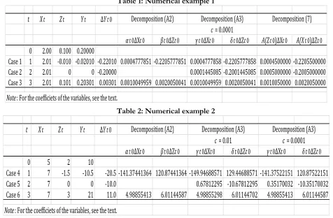
which is not equal to the approximation (A7). The proper discrete approximation may be Eq. (7) in this instance. Table 1: Numerical example 1
Table 2: Numerical example 2
To make up the discussions above, we shall explain the computed results for these decompositions using
strategy replaces a zero-value with a small positive k and this is very different from our Method 2. Their analytical limit strategy is irrelevant to a log-mean. See also [3].
t Xt Zt Yt ΔYt0
αt0ΔXt0 βt0ΔZt0 γt0ΔXt0 δt0ΔZt0 A(Zt0)ΔXt0 A(Xt0)ΔZt0
0 2.00 0.100 0.20000
Case 1 1 2.01 -0.010 -0.02010 -0.22010 0.0004777851 -0.2205777851 0.0004777858 -0.2205777858 0.0004500000 -0.2205500000
Case 2 2 2.01 0 0 -0.20000 0.0001445085 -0.2001445085 0.0005000000 -0.2005000000
Case 3 3 2.01 0.101 0.20301 0.00301 0.0010049959 0.0020050041 0.0010049959 0.0020050041 0.0010050000 0.0020050000
Note: For the coefficiets of the variables, see the text.
Decomposition (A2) Decomposition (A3) Decomposition (7)
c = 0.0001
t
X
tZ
tY
tΔ
Y
t0α
t0ΔX
t0β
t0ΔZ
t0γ
t0ΔX
t0δ
t0ΔZ
t0γ
t0ΔX
t0δ
t0ΔZ
t00
5
2
10
Case 4 1
7
-1.5
-10.5
-20.5 -141.37441364 120.87441364 -149.94688571 129.44688571 -141.37522151 120.87522151
Case 5 2
7
0
0
-10.0
0.67812295 -10.67812295 0.35170032 -10.35170032
Case 6 3
7
3
21
11.0 4.98855413 6.01144587 4.98855298 6.01144702 4.98855413 6.01144587
Note
: For the coefficiets of the variables, see the text.
simple numerical examples. Table 1 shows the results obtained using Eq. (A2), Eq. (A3), and Eq. (7) under the assumption wherein only the variation of X is very small. Conversely, the variation of Z becomes necessarily large when Zs> 0 and Zt≠ s ≤ 0. (Note that Eq. (7) always holds for any real variable.) The two independent variables are given in the table; subscript t (1, 2, or 3) exhibits the comparison period and 0 the base period. The base period is always fixed. For example, ∆𝑌𝑡0 = 𝑌2− 𝑌0, if t = 2. The undefined symbols in the table are
𝛼𝑡0 =𝐿(Φ)𝐴(𝑋)
𝐿(Ψ)𝐴(𝑌), 𝛽𝑡0 =
𝐿(Φ)𝐴(𝑍)
𝐿(Ω)𝐴(𝑌), 𝛾𝑡0 =
𝐴(𝑋)
𝐿(Ψ){
𝐿(Γ)
𝐴(𝑀)+
𝐿(Λ)
𝐴(𝑁)},
𝛿𝑡0= 1
2{
𝐿(Γ)𝐴(𝑈)
𝐿(Θ)𝐴(𝑀)+
𝐿(Λ)𝐴(𝑉)
𝐿(Υ)𝐴(𝑁)} , 𝐴(𝑍𝑡0) = 𝐴(𝑍𝑡, 𝑍0), 𝐴(𝑋𝑡0) = 𝐴(𝑋𝑡, 𝑋0).
Whereas the decomposition of Eq. (A2) cannot apply to Case 2 because of Z2= 0, Eq. (A3) and Eq. (7) can apply to all cases. (In Table 1, we used c =0.0001 for Eq. (A3).) Comparing the computed results using Eq. (A2) with those from Eq. (A3), we find close relationships for Cases 1 and 3. Comparing the results from Eq. (A3) with those from Eq. (7), we see that the two contributions in Cases 1 and 3 are close. In Case 2, however, the X contribution of Eq. (A3) is far removed from that of Eq. (7). The reason why this difference is produced is beyond the scope of this paper. (We presently infer that Eq. (7) in Case 2 cannot be used as the discrete approximation to the AD produced by the differential calculus. See also Appendix B.)
Table 2 shows the computed results using Eq. (A2) and Eq. (A3) without the assumption above. For Eq. (A3), we computed two cases : c = 0.01 and c = 0.0001. Two independent variables are also exhibited in the table. Note that the results from Eq. (A2) in Case 6 are equal to those from Eq. (9). The table shows that the two contributions of Eq. (A3) depend on c. Comparing the results using the smaller c value with those using another value in Cases 4 and 6, we see that the deviations of the former from the results derived using Eq. (A2) are less than those of the latter. Additionally, two X contributions in Case 5 are very different. Recall that a similar behavior is found in Case 2 above.
Appendix B: Comparison of the Difference and Conventional Calculi
We focus on the superior properties of the difference calculus over the conventional calculus using the same examples. Here, only ADs are shown and all variables are positive.
1) Example a: 𝑌𝑡 = 𝑋𝑡𝑍𝑡.
The conventional calculus leads to Eq. (7) and the difference calculus to Eq. (9). To compare the former with the latter, we need to employ two approximations explained in Subsection 4.1. These are
𝐺(𝑥)
𝐴(𝑥)=
𝐺(𝑥1, 𝑥0) 𝐴(𝑥1, 𝑥0)=
𝐺(𝑥1⁄ , 1)𝑥0 𝐴(𝑥1⁄ , 1)𝑥0 =
𝐺(1 + (∆𝑥10⁄ ), 1)𝑥0 𝐴(1 + (∆𝑥10⁄ ), 1)𝑥0 ≈ 1 −
3
24(
∆𝑥10
𝑥0 )
2
𝐺(𝑥)
𝐿(𝑥) =
𝐺(𝑥1, 𝑥0) 𝐿(𝑥1, 𝑥0)≈ 1 −
1
24(
∆𝑥10
𝑥0 )
2
Given that the second-order terms of these approximations are negligible, we have
𝐴(𝑍) ≈ 𝐺(𝑍) = 𝐺(𝑌) 𝐺(𝑋)⁄ ≈ 𝐿(𝑌) 𝐿(𝑋) and 𝐴(𝑋)⁄ ≈ 𝐺(𝑋) ≈ 𝐿(𝑌) 𝐿(𝑍)⁄ .
Thus, if both X1/X0 and Z1/Z0 (and thereforeY1/Y0) are close to 1, the two components in Eq. (7) approach those in Eq. (9). Below, we shall assume similar approximations as given above.
2) Example b: 𝑌𝑡 = 𝑊𝑡𝑋𝑡𝑍𝑡.
For the conventional calculus, we may use transformations of the variables such as 𝐷𝑡 = 𝑋𝑡𝑍𝑡, 𝐸𝑡 =
𝑊𝑡𝑍𝑡, and 𝐹𝑡 = 𝑊𝑡𝑋𝑡. Whenever these are applied to this function, the AD of Eq. (7) derived by the conventional
calculus can be utilized. If we utilize Dt, we obtain the AD by repeatedly utilizing Eq. (7):
∆𝑌10= 𝑊1𝐷1− 𝑊0𝐷0= 𝐴(𝐷)∆𝑊10+ 𝐴(𝑊)∆𝐷10 = 𝐴(𝑋𝑍)∆𝑊10+ 𝐴(𝑊)(𝐴(𝑍)∆𝑋10+ 𝐴(𝑋)∆𝑍10).
∆𝑌10= 𝑎∆𝑊10+ 𝑏∆𝑋10+ 𝑐∆𝑍10, (B1) wherein
𝑎 = (𝐴(𝑋𝑍) + 2𝐴(𝑋)𝐴(𝑍)) 3, 𝑏 =⁄ (𝐴(𝑊𝑍) + 2𝐴(𝑊)𝐴(𝑍)) 3,⁄
𝑐 = (𝐴(𝑊𝑋) + 2𝐴(𝑊)𝐴(𝑋)) 3.⁄
In sharp contrast, our difference calculus can easily yield this AD, the procedures being ∆ log 𝑌10= ∆ log 𝑊10+ ∆ log 𝑋10+ ∆ log 𝑍10,
∴ ∆𝑌10= 𝐿(𝑌)
𝐿(𝑊)∆𝑊10+
𝐿(𝑌)
𝐿(𝑋)∆𝑋10+
𝐿(𝑌)
𝐿(𝑍)∆𝑍10. (B2)
In applying the approximations stated above to the two ADs of Eq. (B1) and Eq. (B2), we find
𝑎 ≈ (𝐺(𝑋𝑍) + 2𝐺(𝑋)𝐺(𝑍)) 3⁄ = 𝐺(𝑋𝑍) = 𝐺(𝑊𝑋𝑍) 𝐺(𝑊) ≈ 𝐿(𝑌) 𝐿(𝑊)⁄ ⁄ , 𝑏 ≈ G(𝑊𝑍) ≈
𝐿(𝑌) 𝐿(𝑋), 𝑐 ≈⁄ 𝐺(𝑊𝑋) ≈ 𝐿(𝑌) 𝐿(𝑍)⁄ .
In passing, we note that the differential calculus establishes the following AD:
d𝑌 = 𝑋𝑍d𝑊 + 𝑊𝑍d𝑋 + 𝑊𝑋d𝑍 = (𝑌 𝑊⁄ )d𝑊 + (𝑌 𝑋⁄ )d𝑋 + (𝑌 𝑍⁄ )d𝑍,
which is closely related to Eq. (B2). See also the correspondences between a finite-change variable and an infinitesimal-change variable in Subsubsection 3.1.3.
The AD derived by the conventional calculus has a shortcoming whenever 𝑊𝑡 = 𝑋𝑡, 𝑋𝑡= 𝑍𝑡, 𝑍𝑡 =
𝑊𝑡, or 𝑊𝑡 = 𝑋𝑡= 𝑍𝑡. We only show an example wherein we assume 𝑋𝑡 = 𝑍𝑡. From Eq. (B1), we obtain
∆𝑌10= (1 3⁄ ) {(𝐴(𝑋2) + 2(𝐴(𝑋))2) ∆𝑊
10
+ 2(𝐴(𝑊𝑋) + 2𝐴(𝑊)𝐴(𝑋))∆𝑍10}.
(B3) Since 𝑌𝑡 = 𝑊𝑡𝐷𝑡 and 𝐷𝑡 = (𝑋𝑡)2, we have another AD from the first-mentioned AD,
∆𝑌10= 𝐴(𝑋2)∆𝑊
10+ 2𝐴(𝑊)𝐴(𝑋)∆𝑋10
= 𝐴(𝑋2)∆𝑊
10+ 2𝐴(𝑊)𝐴(𝑋)∆𝑍10. (B4)
Ordinarily, Eq. (B3) does not equal Eq. (B4).
Contrarily, our differential calculus derives the AD from Eq. (B2), giving
∆𝑌10=
𝐿(𝑌)
𝐿(𝑊)∆𝑊10+ 2
𝐿(𝑌)
𝐿(𝑋)∆𝑋10=
𝐿(𝑌)
𝐿(𝑊)∆𝑊10+ 2
𝐿(𝑌)
𝐿(𝑋)∆𝑍10, (B5)
which is the same as the AD derived using 𝑌𝑡 = 𝑊𝑡(𝑋𝑡)2. The differential calculus analogously leads to the same AD that is given by:
d𝑌 = 𝑋2d𝑊 + 2𝑊𝑋d𝑋 = (𝑌 𝑊⁄ )d𝑊 + (2𝑌 𝑋⁄ )d𝑍. (B6)
It is important that both Eq. (B4) and Eq. (B5) always correspond to Eq. (B6) but Eq. (B3) does not. Therefore, the conventional method cannot always produce the ADs that correspond to those derived by the differential one for multiplicative functions composed of three or more independent variables. The same can be found for the next example, if 𝑋𝑡 = 𝑍𝑡.
3) Example c: 𝑌𝑡= 𝑊𝑡/(𝑋𝑡𝑍𝑡), wherein 𝑊𝑡 ≠ 𝑋𝑡 and 𝑊𝑡 ≠ 𝑍𝑡.
The conventional calculus also exploits the variable transformations, 𝐼𝑡 = 𝑋𝑡𝑍𝑡, 𝐽𝑡 = 𝑊𝑡/𝑍𝑡, and 𝐾𝑡= 𝑊𝑡/𝑋𝑡. These lead to
𝑌𝑡 = 𝑊𝑡⁄ = 𝐽𝐼𝑡 𝑡⁄𝑋𝑡 = 𝐾𝑡⁄ . 𝑍𝑡
Hence, ADs of Eq. (7) and Eq. (8) can be utilized. We obtain, for example, the following using Kt:
∆𝑌10=
𝐾1
𝑍1−
𝐾0
𝑍0 =
𝐾1𝑍0− 𝐾0𝑍1
𝑍1𝑍0 =
𝐴(𝑍)∆𝐾10− 𝐴(𝐾)∆𝑍10
𝑍1𝑍0 ,
∆𝐾10=𝑊1
𝑋1 −
𝑊0
𝑋0 =
𝐴(𝑋)∆𝑊10− 𝐴(𝑊)∆𝑋10
𝑋1𝑋0 .
conventional calculus; specifically,
∆𝑌10=𝑑∆𝑊10− 𝑒∆𝑋10− 𝑓∆𝑍10
𝑋1𝑋0𝑍1𝑍0 ,
where in d, e, and f are
𝑑 = (𝐴(𝑋𝑍) + 2𝐴(𝑋)𝐴(𝑍)) 3,⁄ 𝑒 = (𝑍1𝑍0𝐴(𝑊 𝑍⁄ ) + 2𝐴(𝑊)𝐴(𝑍)) 3⁄ ,
𝑓 = (𝑋1𝑋0𝐴(𝑊 𝑋⁄ ) + 2𝐴(𝑊)𝐴(𝑋)) 3⁄ .
Our difference calculus quickly yields this AD, which is
∆ log 𝑌10= ∆ log 𝑊10− ∆ log 𝑋10− ∆ log 𝑍10,
∴ ∆𝑌10= 𝐿(𝑌)
𝐿(𝑊)∆𝑊10−
𝐿(𝑌)
𝐿(𝑋)∆𝑋10−
𝐿(𝑌) 𝐿(𝑍)∆𝑍10.
If we can apply the above-stated approximations to the two ADs, we find the correspondences between the two methods.
The differential calculus leads to the AD:
d𝑌 = 1
𝑋𝑍d𝑊 −
𝑊
𝑋2𝑍d𝑋 −
𝑊
𝑋𝑍2d𝑍 =
𝑌
𝑊d𝑊 −
𝑌
𝑋d𝑋 −
𝑌
𝑍d𝑍.
We can also find a close relation between the ADs derived by the differential and the difference calculi.
Now, we say that the conventional calculus is senseless for the functions in Example b and Example c.18 How about 𝑌𝑡 = 𝑉𝑡𝑊𝑡/(𝑋𝑡𝑍𝑡)? Although our difference calculus can quickly derive this AD, the conventional calculus needs more awkward and complicated procedures than the above. Additionally, the foregoing discussions and those explained in Subsubsection 3.1.3 make clear that the results derived by our difference calculus are superior to those by the conventional calculus as discrete approximations to those by the differential calculus.
References
[1] Ang, B. W., & Liu, F. L. (2001). A new energy decomposition method: Perfect in decomposition and consistent in aggregation. Energy, 26, 537–548.
[2] Ang, B. W., & Liu, N. (2007a). Handling zero values in the logarithmic mean Divisia index decomposition approach. Energy Policy, 35, 238–246.
[3] Ang, B. W., & Liu, N. (2007b). Negative-value problems of the logarithmic mean Divisia index decomposition approach. Energy Policy, 35, 739–742.
[4] Balk, B. M. (2002–3). Ideal indices and indicators for two or more factors. Journal of Economics and Social Measurement,
28, 203–217.
[5] Balk, B. M. (2008). Price and quantity index numbers: Models for measuring aggregate change and difference. New York: Cambridge University Press.
[6] Bhatia, R. (2008). The logarithmic mean. Resonance, 13(6), 583–594.
[7] Boole, G. (1958). Calculus of finite differences (4th ed.) edited by J. F. Moulton. New York: Chelsea Publishing Company. (Previous editions published under title: A treatise on the calculus of finite differences. The first edition was appeared in 1860.)
[8] Carlson, B. C. (1972). The logarithmic means. American Mathematical Monthly, 79(6), 615–618.
[9] Diewert, W. E. (2005). Index number theory using differences rather than ratios. American Journal of Economics and
Sociology, 64, 311–360.
[10] Dodd, E. L.(1941). Some generalizations of the logarithmic mean and of similar means of two variates which become indeterminate when the two variates are equal. Annals of Mathematical Statistics, 12, 422–428.
[11] Encyclopedia of Mathematics, “Finite-difference calculus, Computational mathematics, Numerical analysis.” [Online] Available: https://www.encyclopediaofmath.org. [Accessed February 13, 2018]
[12] Goldberg, S. (1958). Introduction to difference Equations. New York: John Wiley & Sons.
[13] Jia, G., & Cao, J. (2003). A new upper bound of the logarithmic mean. Journal of Inequalities in Pure and Applied
Mathematics, 4(4), 1–4.
[14] Jordan, C. (1965). Calculus of finite differences (3rd ed.). New York: Chelsea Publishing Company.
[15] Paterson, W. R. (1984). A replacement for the logarithmic mean. Chemical Engineering Science, 39(11), 1635–1636. [16] Pittenger, A. O. (1985). The logarithmic mean in n variables. American Mathematical Monthly, 92(2), 99–104. [17] Spiegel, M. R. (1971). Theory and problems of calculus of finite differences and difference equations. New York: McGraw-Hill. [18] Stolarsky, K. B. (1975). Generalizations of the logarithmic mean. Mathematics Magazine, 48(2), 87–92.
[19] Sugano, H., & Tsuchida, S. (2002). A new approach to discrete data (in Japanese). Bulletin, Faculty of Business
Information Sciences, Jobu University, 1, 29–55.
[20] Tsuchida, S. (1997). A family of almost ideal log-change index numbers. Japanese Economic Review, 48, 324–342. [21] Tsuchida, S. (2014). Interconvertible rules between an aggregative index and a log-change index. Electronic Journal
of Applied Statistical Analysis, 7 (2), 394–415. [Online] Available:
http://siba-ese.unisalento.it/index.php/ejasa/issue/view/1259.
[22] Tsuchida, S. (2015). Strategic decomposition: How to increase total labor productivity. International Journal of
Contemporary Economics and Administrative Sciences, 5 (3–4), 109–138.
[23] Vartia, Y. O. (1976). Ideal log-change index numbers. Scandinavian Journal of Statistics, 3, 121–126.
[24] Zhao, Y., Liu, Y., Zhang, Z., Wang, S., Li, H., & Ahmad, A. (2017). CO2 emissions per value added in exports of China: A comparison with USA based on generalized logarithmic mean Divisia index decomposition. Journal