Vol. 11, No. 1, 2019 Article ID IJIM-0920, 8 pages Research Article
An Efficient Numerical Method for a Class of Boundary Value
Problems Based on Shifted Jacobi-Gauss Collocation Scheme
M. Maleki Miyane ∗, S. Abbasbandy †‡
Received Date: 2016-08-06 Revised Date: 2017-02-23 Accepted Date: 2017-07-09
————————————————————————————————–
Abstract
This paper proposes a numerical method to deal with the two-dimensional hyperbolic equations with nonlocal integral conditions. The nonlocal integral equation usually is of major challenge in the frame work of the numerical solutions of partial differential equations. The method benefits from collocation radial basis function method, the generalized thin plate splines (GTPS) radial basis functions are used. Therefore, it does not require any struggle to determine shape parameter (In other RBFs, it is time-consuming step). The present technique is one of the truly meshless methods in where it does not require any background integration cells over local or global domains and it is in contrast to weak form methods in where all integrations are carried out locally or globally over quadrature domains of regular shapes, such as lines in one dimensions, circles or squares in two dimensions and spheres or cubes in three dimensions. The obtained results for some numerical examples reveal that the proposed technique is very effective, convenient and quite accurate to such considered problems.
Keywords: Collocation method; Shifted Jacobi polynomial; Singular boundary value problem; Expo-nential nonlinearity; Product nonlinearity.
—————————————————————————————————–
1
Introduction
S
pods of discretization for the numerical solu-ectral methods are one of the principal meth-tion of boundary value problems, initial value problems and so on [1,2,3,4,5]. The most widely used spectral versions are the Galerkin, colloca-tion, and Tau methods [6]. Collocation methods are very popular for solving such problems, also they are very applicable in providing highlyac-∗Department of Applied Mathematics, Imam Khomeini
International University, Qazvin, Iran.
†Corresponding author. [email protected],
Tel:+98(912)1305326.
‡Department of Applied Mathematics, Imam Khomeini
International University, Qazvin, Iran.
curate solutions to these problems. In this paper, we extended the application of Jacobi polynomi-als from Galerkin method for solving nonlinear second-order initial value problems (see [7,8]) to collocation method to solve a class of boundary value problems on the unit interval which feature a type of exponential and product nonlinearities.
A well-known advantage of a spectral method is that it achieves high accuracy with relatively fewer spatial grid points in comparison by a finite-difference method. Also, in using spectral meth-ods, we meet to full matrices, partially negating the gain in efficiency due to the fewer number of grid points (see [9,10]). The use of Jacobi polyno-mials has the advantage of obtaining the solutions of nonlinear differential equations, [8,11].
The fundamental goal of this paper is com-parison of the result of the numerical solution of boundary value problem (BVP) by collocation methods with Adomian Decomposition Method (ADM) and Reproducing Kernel Method (RKM) and we will observe that present method is both efficient and accurate.
The BVP is collocated only at nodes of the shifted Jacobi-Gauss interpolation as collocation points. The main equation together with initial conditions generate a system of algebraic equa-tions which can be solved using Newton’s itera-tive method.
This paper is organized as follows. In Section
2, an overview of shifted Jacobi polynomials and their relevant properties needed hereafter is pre-sented. In Section 3, we construct the colloca-tion method by using the shifted Jacobi polyno-mials in two cases, for a two-point boundary value problem for the fourth-order nonlinear differential equation with an exponential nonlinearity, for a two-point boundary value problem for the fourth-order nonlinear differential equation with a prod-uct nonlinearity, respectively. In Section 4, we present some numerical results exhibiting the ac-curacy and efficiency of our numerical algorithms, and a brief conclusion in Section 5.
2
Preliminaries
Let α >−1, β >−1, and Pn(α,β)(r) be the stan-dard Jacobi polynomial of degree n. Obviously, we have
Pn(α,β)(−r) = (−1)nPn(α,β)(r),
Pn(α,β)(−1) = (−1)
nΓ(n+β+ 1)
n! Γ(β+ 1) ,
Pn(α,β)(1) = Γ(n+α+ 1)
n! Γ(α+ 1) . (2.1)
The m-th derivative ofPn(α,β)(r) is defined as
DmPn(α,β)(r) =
2−mΓ(m+n+α+β+ 1) Γ(n+α+β+ 1) P
(α+m,β+m)
n−m (r). (2.2)
The set of Jacobi polynomials with the weight function ω(α,β)(r) = (1 −r)α(1 + r)β forms a weighted Hilbert space L2ω(α,β)[−1,1], which is
also a complete system by standard inner prod-uct. The shifted Jacobi polynomial of degree n
is defined by Jn(α,β)(r) = Pn(α,β)(2r −1), and by using (2.1) and (2.2), it can be shown that
DmJn(α,β)(r) =
Γ(m+n+α+β+ 1) Γ(n+α+β+ 1) J
(α+m,β+m)
n−m (r). (2.3)
The set of shifted Jacobi polynomials with the weight function χ(α,β)(r) = (1−r)αrβ forms a weighted Hilbert space L2χ(α,β)[0,1], which is also a complete system by standard inner product. Moreover, we have
∥Jn(α,β)∥2χ(α,β)=
(1 2
)α+β+1
∥Pn(α,β)∥2ω(α,β).
The symmetric Jacobi polynomials, the shifted Chebyshev of the first kind, the shifted Cheby-shev of the second kind and the shifted Legendre polynomials are recovered by α = β, α = β = −0.5,α=β = +0.5,α=β = 0, respectively.
The nodes of the standard Jacobi-Gauss in-terpolation on the interval [−1,1] and their cor-responding Christoffel numbers are denoted by
rN,j(α,β) and ϖN,j(α,β), 0 ≤ j ≤ N, respectively.
We denote by θ(N,jα,β), 0 ≤ j ≤ N the nodes of the shifted Jacobi-Gauss interpolation on [0,1], which are the zeros of JN(α,β+1). It can be shown
θ(N,jα,β) = (r(N,jα,β) + 1)/2 and their corresponding
Christoffel numbers are ϑ(N,jα,β) = (12)α+β+1ϖN,j(α,β)
forj = 0,1, . . . , N. By the properties of the stan-dard Jacobi-Gauss quadrature, if ϕ be a polyno-mial of degree at most 2N + 1, we have [7]
∫ 1
0
(1−r)αrβϕ(r)dr
= N ∑
j=0
ϑ(N,jα,β)ϕ(θ(N,jα,β)).
In practice, only the first (N + 1) terms shifted Jacobi polynomials are considered.
3
Shifted Jacobi-Gauss
Colloca-tion Method
a class of boundary value problems on the unit interval which feature a type of exponential and product nonlinearities.
3.1 Exponential nonlinearity
Consider the two-point boundary value problem for the fourth-order nonlinear differential equa-tion with an exponential nonlinearity [13]
u′′′′(r) + 6e−4u(r)= 0, r ∈[0,4−e], (3.4)
subject to
u(0) = 1, u′′(0) =−1
e2,
u(4−e) = ln(4), u′′(4−e) =− 1
16. (3.5)
One of the important step in the collocation method is the choice of collocation points which effect on efficiency. Let us first introduce some basic notation. We set
SN(0,1) =span{J0(α,β)(r), J (α,β) 1 (r), ...,
JN(α,β)(r)} (3.6)
and we define the discrete inner product and norm as follows:
(u, v)χ(α,β),N = N ∑
j=0
u(θ(N,jα,β))v(θN,j(α,β))ϑ(N,jα,β),
(3.7)
∥u∥χ(α,β),N= √
(u, v)χ(α,β),N.
Here θN,j(α,β) and ϑ(N,jα,β) are the nodes and the cor-responding weights of the shifted Jacobi-Gauss quadrature formula on the interval (0,1), respec-tively. Obviously,
(u, v)χ(α,β),N = (u, v)χ(α,β), ∀u, v∈S2N−1. (3.8) Thus, for anyu∈SN(0,1), the norms∥u∥χ(α,β),N and ∥u∥χ(α,β) are equal.
Associating with this quadrature rule, we de-note by INJ(α,β) the shifted Jacobi-Gauss interpo-lation,
INJ(α,β)u(θ(N,jα,β)) =u(θ(N,jα,β)), 0≤j≤N. (3.9)
The shifted Jacobi-Gauss collocation method for solving (3.4) and (3.5) is to seek vN(x) ∈
SN(0,1), such that
u′′′′(θN,j(α,β)) + 6e−4u(θ(N,jα,β))= 0, (3.10)
j = 0,1, ..., N,
uN(0) = 1, u′′N(0) =− 1
e2,
uN(4−e) = ln(4), u′′N(4−e) =− 1 16.
We now derive an algorithm for solving (3.5) and (3.4). To do this, let
uN(r) = N ∑
j=0
ajJj(α,β)(r),
a= (a0, a1, ..., aN)T. (3.11)
We first approximateu(r), u′(r), u′′(r) , as (3.11). By substituting these approximation in (3.4), we get
N ∑
j=0
ajD4Jj(α,β)(r)
+ 6e−4
∑N
j=0ajJj(α,β)(r)= 0. (3.12)
Then, by virtue, we deduce that
N ∑
j=0
ajcj1cj2cj3cj4Jj(−α+44 ,β+4)(r) (3.13)
+ 6e−4∑Nj=0ajJ (α,β)
j (r) = 0,
where cji=α+β+j+i.
Also, by substituting (3.11) in (3.5) we obtain
N ∑
j=0
ajJj(α,β)(0) = 1,
N ∑
j=0
ajD2Jj(α,β)(0) =− 1
e2,
N ∑
j=0
ajJj(α,β)(4−e) = ln(4),
N ∑
j=0
ajD2Jj(α,β)(4−e) =− 1
To find the solution uN(r), we first collocate (3.13) at the Jacobi rational roots, yielding
N ∑
j=0
ajcj1cj2cj3cj4Jj(−α+44 ,β+4)(r)
+ 6e−4∑Nj=0ajJj(α,β)(r)= 0. (3.15)
Equation (3.14), after using of virtue of Shifted Jacobi-Gauss polynomial, can be written as
N ∑
j=0
(−1)jΓ(j+β+ 1)
Γ(j+ 1)Γ(β+ 1) aj −1 = 0,
N ∑
j=0
(−1)j−2cj1cj2Γ(j+β+ 1)
Γ(j−1)Γ(β+ 3) aj+ 1
e2 = 0,
N ∑
j=0
Γ(j+α+ 1) Γ(j+ 1)Γ(cj1)×
j ∑
s=0
Γ(cj1+s)
Γ(α+s+ 1)(3−e) sa
j −ln(4) = 0,
N ∑
j=0
Γ(j+α+ 1) Γ(j−1)Γ(cj3)×
j ∑
s=0
Γ(cj3+s)
Γ(α+s+ 3)(3−e) sa
j+ 1
16 = 0. (3.16)
Finally, from (3.15) and (3.16), we get a system of nonlinear algebraic equations which can be solved for the unknown coefficientsajby using any stan-dard iteration technique, like Newton’s iteration method. Consequently,uN(r) given in (3.11) can be evaluated.
3.2 Product nonlinearity
Consider the two-point boundary value problem for the fourth-order nonlinear differential equa-tion with a product nonlinearity [12,13]
u′′′′(r) +u(r)u′(r)−4r7−24 = 0, r ∈[0,1],
(3.17) subject to
u(0) = 0, u′′′(0.25) = 6,
u′(0.5) = 3, u(1) = 1. (3.18)
The shifted Jacobi-Gauss collocation method for solving (3.17) and (3.18) is to seek vN(x) ∈
SN(0,1), such that
u′′′′(θN,j(α,β)) +u(θN,j(α,β))u′(θ(N,jα,β))
−4(θN,j(α,β))7−24 = 0, j= 0,1, ..., N, uN(0) = 0, u′′′N(0.25) = 6,
u′N(0.5) = 3, uN(1) = 1. (3.19) We now derive an algorithm for solving (3.17) and (3.18). To do this, let
uN(r) = N ∑
j=0
ajJj(α,β)(r), a= (a0, a1, ..., aN)T.
(3.20) We first approximateu(r), u′(r), u′′(r), as (3.20). By substituting these approximation in (3.17), we get
N ∑
j=0
ajD4J(α,β)Jj(r)
+ N ∑
j=0
ajJ(α,β)Jj(r) N ∑
j=0
ajDJ(α,β)Jj(r)
−4r7−24 = 0. (3.21) Then, by virtue, we deduce that
N ∑
j=0
ajcj1cj2cj3cj4J(α,β)Jj(−α+44 ,β+4)(r)
− N ∑
j=0
ajJ(α,β)Jj(α,β)(r)×
N ∑
j=0
ajcj1ajJ(α,β)Jj(α−+11 ,β+1)(r)
−4r7−24 = 0. (3.22) Also, by substituting (3.20) in (3.18) we obtain
N ∑
j=0
ajJj(α,β)(0) = 0,
N ∑
j=0
ajD3Jj(α,β)(0.25) = 6,
N ∑
j=0
ajD2Jj(α,β)(0.5) = 3,
N ∑
j=0
To find the solution uN(r), we first collocate (3.22) at the Jacobi rational roots, yielding
N ∑
j=0
ajcj1cj2cj3cj4J(α,β)Jj(−α+44 ,β+4)(r)
− N ∑
j=0
ajJ(α,β)Jj(α,β)(r)×
N ∑
j=0
ajcj1J(α,β)Jj(−α+11 ,β+1)(r)
−4r7−24 = 0. (3.24)
Equation (3.23), after using of virtue of Shifted Jacobi-Gauss polynomial, can be written as
N ∑
j=0
(−1)jΓ(j+β+ 1)
Γ(j+ 1)Γ(β+ 1) aj = 0,
N ∑
j=0
cj1cj2Γ(j+α+ 1)
Γ(j−1)Γ(cj3) ×
j ∑
s=0
Γ(cj3+s)
Γ(α+s+ 3)(−0.75) sa
j−6 = 0,
N ∑
j=0
cj1cj2Γ(j+α+ 1)
Γ(j−1)Γ(cj3) ×
j ∑
s=0
Γ(cj3+s)
Γ(α+s+ 3)(−0.5) sa
j −3 = 0,
N ∑
j=0
Γ(j+α+ 1)
Γ(j+ 1)Γ(α+ 1)aj = 0. (3.25)
Finally, from (3.24) and (3.25), we get a system of nonlinear algebraic equations which can be solved for the unknown coefficientsajby using any stan-dard iteration technique, like Newton’s iteration method. Consequently,uN(r) given in (3.20) can be evaluated.
4
Numerical Examples
In this section, we have a comparison between the proposed method explained in pervious sections and some other numerical methods in solving lin-ear and nonlinlin-ear differential equations. This comparison shows the validity and applicability of our proposed method.
Example 4.1 Consider the two-point boundary value problem for the fourth-order nonlinear dif-ferential equation with an exponential nonlinear-ity (3.4) and (3.5), [13, 14]. The exact solution of this problem is u(x) = ln(e + x).
The best error obtained in [13] by ADM is 2.3×10⁻⁵, approximately. Also, the best error
obtained in [14] by RKM is 5.8×10⁻⁸. The ab-solute errors|u(r)−uN(r)|, reported in Table1, show the accuracy of the present method.
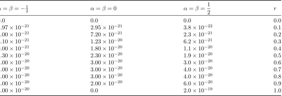
Example 4.2 Consider the two-point bound-ary value problem for the fourth-order nonlinear differential equation with a product nonlinearity (3.17) and (3.18), [12, 13, 14]. The exact solu-tion of this problem is u(r) =r4.
This problem is consider in [12] by Adomian de-composition method (ADM), and in [13] by mod-ified Adomian decomposition method (MADM). The best error obtained in [12] is 1.0×10⁻¹⁰, and in [13] is 5.4×10⁻⁹, approximately. Also, the best
error obtained in [14] by RKM is 2.2×10⁻¹⁴. The absolute errors |u(r)−uN(r)|, reported in Table
2, show the accuracy of the present method.
Example 4.3 Consider the following singular fourth order four-point boundary value problem [14, 15]
sin(r)(er−1)2u′′′′(r) + 300er2u′(r) + 200 sin(√r)u′′(r) +rsinh(r)u′(r) +rsin(u(r)) =f(r), r∈[0,1],
u(0) = 0, u(1
3) = sin( 1 3),
u(2
3) = sin( 2
3), u(1) = sin(1),
where
f(r) = (−1 +er)2sin2(r)−2 sin(√r) sin(r) −er2 cos(r) +rsin(sin(r)) + cos(r) sinh(r).
The exact solution of this problem is u(r) = sin(r).
Table 1: Absolute errors withN = 31 for Example4.1.
α=β=−12 α=β= 0 α=β =1
2 r
1.×10−20 3.×10−20 1.×10−19 0.0
7.9516053250797606810×10⁻²³ 3.3434710028806590559×10⁻²² 3.9392630304801456252×10⁻²² 0.1
2.0000006108250784288×10⁻¹⁹ 1.0000215024548864886×10⁻¹⁹ 2.0000149618669976087×10⁻¹⁹ 0.2
2.2751751705451664619×10⁻²² 9.5176590214182709569times10−22 2.0000316084519611054×10⁻¹⁹ 0.3
1.0000042129860206793×10⁻¹⁹ 1.2097647203036968936×10⁻²¹ 3.0000341664421918505×10⁻¹⁹ 0.4
1.0000058389525492761×10⁻¹⁹ 1.4172826887112441484×10⁻²¹ 1.0001412930681577235×10⁻¹⁹ 0.5
1.0000071832906491791×10⁻¹⁹ 1.0001219615783720258×10⁻¹⁹ 2.0000862855539263074×10⁻¹⁹ 0.6
1.0000079738265055987×10⁻¹⁹ 1.0001330048377446228×10⁻¹⁹ 2.0000948144228097547×10⁻¹⁹ 0.7 3.9983394948964359366×10⁻²² 1.6124273746517058476×10⁻²¹ 1.9355975958912418494×10⁻²¹ 0.8 1.0000071268506422337×10⁻¹⁹ 1.4938250446988961272×10⁻²¹ 5.0000326781265528444×10⁻¹⁹ 0.9 1.0000054021297995555×10⁻¹⁹ 1.0000799115193710960×10⁻¹⁹ 2.0000599932646300490×10⁻¹⁹ 1.0
Table 2: Absolute errors withN = 7 for Example4.2.
α=β=−12 α=β= 0 α=β= 1
2 r
0.0 0.0 0.0 0.0
1.97×10⁻²¹ 2.95×10⁻²¹ 3.8×10⁻²² 0.1
4.00×10⁻²¹ 7.20×10⁻²¹ 2.3×10⁻²¹ 0.2
6.10×10⁻²¹ 1.23×10⁻²⁰ 6.2×10⁻²¹ 0.3
9.00×10⁻²¹ 1.80×10⁻²⁰ 1.1×10⁻²⁰ 0.4
1.30×10⁻²⁰ 2.30×10⁻²⁰ 1.9×10⁻²⁰ 0.5
1.00×10⁻²⁰ 3.00×10⁻²⁰ 3.0×10⁻²⁰ 0.6
1.00×10⁻²⁰ 3.00×10⁻²⁰ 4.0×10⁻²⁰ 0.7
2.00×10⁻²⁰ 3.00×10⁻²⁰ 4.0×10⁻²⁰ 0.8
3.00×10⁻²⁰ 2.00×10⁻²⁰ 6.0×10⁻²⁰ 0.9
3.00×10⁻²⁰ 0.0 2.0×10⁻¹⁹ 1.0
Table 3: Absolute errors withN = 11 for Example4.3.
α=β=−1
2 α=β = 0 α=β =
1
2 r
1.×10−20 1.×10−20 1.×10−20 0.0
3.5807×10⁻¹⁷ 2.12286×10⁻¹⁶ 6.59712×10⁻¹⁶ 0.1
4.509×10⁻¹⁷ 1.0000×10⁻¹⁶ 3.4955×10⁻¹⁶ 0.2
6.495×10⁻¹⁷ 3.786×10⁻¹⁷ 1.02×10⁻¹⁸ 0.3
4.104×10⁻¹⁷ 5.371×10⁻¹⁷ 1.1417×10⁻¹⁶ 0.4
2.3349×10⁻¹⁶ 2.7981×10⁻¹⁶ 5.0367×10⁻¹⁶ 0.5
3.423×10⁻¹⁷ 2.527×10⁻¹⁷ 1.6451×10⁻¹⁶ 0.6
1.4038×10⁻¹⁶ 1.3110×10⁻¹⁶ 1.7176×10⁻¹⁶ 0.7
4.9256×10⁻¹⁶ 7.7813×10⁻¹⁶ 1.63389×10⁻¹⁵ 0.8
6.9288×10⁻¹⁶ 1.24280×10⁻¹⁵ 2.63556×10⁻¹⁵ 0.9
1.0×10⁻¹⁹ 0.0 6.0×10⁻²⁰ 1.0
5
Conclusions
In this article, we have proposed a numerical algo-rithm to solve a class of boundary value problems. The Shifted Jacobi-Gauss collocation method was
equa-tions which can be solved using Newtons iterative method. Numerical results were given to show the accuracy and applicability of the presented method. The method is rather robust, hence it may be applied to other type of singular non-linear boundary value problems with more com-plicated forms of nonlinearity.
References
[1] C. Canuto, M. Y. Hussaini, A. Quarteroni, and T. A. Zang, Spectral Methods in Fluid Dynamics, Springer, New York, NY, USA, 1988.
[2] B. Fornberg, A Practical Guide to Pseu-dospectral Methods,Vol. 1, Cambridge Uni-versity Press, Cambridge, UK,1998.
[3] R. Peyret, SpectralMethods for Incompress-ible Viscous Flow, Vol. 148, Springer, New York, NY, USA,2002.
[4] L. N. Trefethen, Spectral Methods in MAT-LAB, Vol. 10, SIAM, Philadelphia, Pa, USA,2000.
[5] S.Gh. Hosseini, E. Babolian, S. Abbasbandy, A new algorithm for solving Van der Pol equation based on piecewise spectral Ado-mian decomposition method, Int. J. Indus-trial Mathematics 8 (2016) 177-184.
[6] J. Shen, T. Tang, L. L.Wang, Spectral Meth-ods: Algorithms, Analysis and Applica-tions, Vol. 41 of Springer Series in Compu-tational Mathematics, Springer, Heidelberg, Germany,2011.
[7] A. H. Bhrawy, A. S. Alofi, R. A. Van Gorder, An efficient collocation method for a class of boundary value problems arising in math-ematical physics and geometry, Abs. Appl. Anal., Vol. 2014,Article ID 425648, 2014.
[8] A. H. Bhrawy, M. A. Alghamdi, A shifted Jacobi-Gauss collocation scheme for solv-ing fractional neutral functional-differential equations, Adv. Math. Phys., vol. 2014, Ar-ticle ID 595848, 2014
[9] S. Abbasbandy, H. Roohani Ghehsareh, I. Hashim, An approximate solution of the MHD flow over a non-linear stretching sheet by rational Chebyshev collocation method, Univ. Politehn. Bucharest Sci. Bull. Ser. A 74 (2012) 47-58.
[10] S. Abbasbandy, T. Hayat, H. Roohani Ghehsareh, A. Alsaedi, MHD Falkner-Skan flow of Maxwell fluid by rational Chebyshev collocation method,Appl. Math. Mech. Engl. Ed. 34 (2013) 921-930.
[11] E. H. Doha, A. H. Bhrawy, W. M. Abd-Elhameed, Jacobi spectral Galerkin method for elliptic Neumann problems, Numerical Algorithms 50 (2009) 67-91.
[12] M. Tatari, M. Dehghan, The use of the Ado-mian decomposition method for solving mul-tipoint boundary value problems,Phys. Scr. 73(2006)672-676.
[13] J. S. Duan, R. Rach, A new modification of the Adomian decomposition method for solving boundary value problems for higher order nonlinear differential equations, Appl. Math. Comput.218 (2011)4090-4118.
[14] M. Q. Xu, Y. Z. Lin, Y. H. Wang, A new algorithm for nonlinear fourth order multi-point boundary value problems,Appl. Math. Comput.274 (2016) 163-168.
[15] X. Y. Li, B. Y. Wu, A novel method for nonlinear singular fourth order four-point boundary value problems, Comput. Math. Appl.62 (2011) 27-31.