An Additive Model for Estimation Return to Scale in Regulated Environment with Quasi-Fixed Inputs in Data Envelopment Analysis (DEA)

(1)

893

Available online at http://ijdea.srbiau.ac.ir

Int. J. Data Envelopment Analysis (ISSN 2345-458X)

Vol.4, No.1, Year 2016 Article ID IJDEA-00412, 9 pages

Research Article

An Additive Model for Estimation Return to Scale in

Regulated Environment with Quasi-Fixed Inputs in

Data Envelopment Analysis (DEA)

Farshid Emami

a*

, Toktam Nasirzade Tabrizi

b

(a) Department of Mathematics, Shahid Rajaee Teacher Training University, Lavizan, Tehran, Iran.

(b)

Department of Mathematics, Science and Research Branch,

Islamic Azad University.

Received 28 February 2016, Revised 27 May 2016, Accepted 20 June 2016

Abstract

The measurement of RTS amounts measures a relationship between inputs and outputs in a production structure. There are many different ways to calculate RTS in primal or dual space. But in more realistic cases, governments usually intervene on DMU’s behavior as regulatory agency, this clearly represent a set of limitations and restrictions on behaviors of DMUs, So very few decisions in DMUs are made without intersecting some regulations. Therefore it is essential to be able to assess the impact of regulation on the behavior of the DMUs, and this would be ideally done by estimating returns to scale with and without the effect of the regulation.

In this paper we use additive model to provide an alternative approach for estimating returns to scale in regulated environments. The proposed model is developed to determining returns to scale in the presence of quasi-fixed inputs in Data Envelopment Analysis.

Keywords:

Returns to scale, Regulation, Quasi-fixed inputs.

*_{Corresponding Author: [email protected]}

(2)

894

1. Introduction

Measuring the efficiency of a decision making unit (DMU) has long been considered as a difficult task because one is dealing with complex economic and behavioral entities. This task becomes more difficult when it involves multiple inputs and multiple outputs. Data Envelopment Analysis (DEA) is a managerial powerful tool to evaluate the relative efficiency of each decision making unit. It was introduced by Charnes et al in 1978, with CCR model [1].

For a DMU, the production process is to consume the inputs to get the outputs, and the efficiency is to obtain more outputs with fewer

inputs as much as possible. A number of

different DEA models have now appeared in the literature for efficiency measurement. It should be noted that in the production process all the inputs and outputs can be varied at the discretion of management or other users. These may be called “discretionary variables.” But “Non-discretionary variables,” not being subject to management control, may also need to be considered. The conceptual meaning of non-discretionary inputs contains a big class of variables our focus here is on inputs. For example the number of faculties of a university can be considered as non-discretionary inputs. Banker and Morey (1986) introduced non-discretionary inputs [2] and after that Charnes et al 1987 extended the additive model in order to accommodate non-discretionary variables [3].

One of the most important concepts in the theory of production is the scale of operations

(RTS). It can provide beneficial information about the size of DMUs. RTS in DEA was introduced by Banker (1984) [4]. Since then, there have been many attempts to evaluate RTS

within the DEA context. For example, Banker

et al [5] provided an approach based on supporting hyperplane. Fare and Grosskopf [6] provided an alternative approach to estimate returns to scale which is based on optimal solutions of BCC, CCR, and CCR-BCC models. In a more realistic environment of the DMUs, not all inputs are fully discretionary and the environment in which they operate is regulated, Ouellette et al (2012) [7] showed how to introduce these refinements of the firm’s environment into the calculation of RTS. They consequently introduced regulations as an important part of the DMU΄s environment. The focus of this paper is on estimating returns to scale for DEA models when DMUs face a complex environment that includes regulation and quasi-fixed inputs.

It is noteworthy that, since an inefficient DMU has more than one projection on the empirical function hence, different returns to scales can be obtained for projections of the inefficient DMU by using the proposed approach.

2. Preliminaries

In this section, BCC model for estimating returns to scale in DEA is described.

Production possibility set (PPS) is defined as PPS = {(X,Y) | Y 0 can be produced by X 0} and here supposed that PPS = PPSBCC

(3)

895

= PPSBCC , | ∑ ,

∑ , ∑ 1 , 0 , 1, … .

Let α (β) = max {α|(βx, α , (†) Banker defines and as bellows:

lim , lim

Now according to definition of , , the following theorem identify quality of RTS for

.

Theorem 1 Suppose that then

1 1

.

1 1

.

1 1

.

To use the BCC model to calculate the returns to scale, Suppose we have n DMUs in which ( : 1, … , ) use m inputs

1, … , to produce s outputs

1, . . , . Moreover, the BCC multiplier model

for efficiency evaluated of .is as

follows:

Max ∑

s.t ∑ 1 (1)

∑ ∑ 0

1, … 0 و 0

Now suppose that ( , , be an optimal solution for model (1). Banker and Thrall presented the following theorem for estimatingRTS of BCC-efficient DMUs[8]

Theorem 2. Suppose that (x , y ) is a point on

the BCC-efficient frontier. Then, the following

conditions identify the situation for RTS at the point:

(i) Increasing RTS (IRS) prevail at ( , ) if and only if 0 for all optimal solutions of model (1).

(ii) Decreasing RTS (DRS) prevail at ( , ) if and only if 0 for all optimal solutions of model(1)

(iii) Constant RTS (CRS) prevail at ( , ) if and only if 0 for at least one optimal solution of model (1).

2.1 Khodabakhshi et al. model to estimate

returns to scale.

Khodabakhshi et al provided a DEA approach to calculate the returns to scale based on additive model as follows:

Suppose that DMUO is a BCC-efficient DMU

and consider the following additive model that has been presented by Charnes et al. [9] to evaluate the DMUo:

Max ∑ ∑

s.t. ∑ i=1,2,…,m ∑ r=1,2,…,s ∑ 1 (2) 0 j=1,2,…,n

, 0

Definition 2. DMUo is called efficient if and

only if the obtained optimal value of objective function from model (3) is zero.

Theorem3. Suppose that DMUo with input–

output combination ( , ) is efficient. Therefore, we have:

(i) There is ξ>1 so that ,

(4)

896

(ii) There is 0<ξ<1 so that , is inefficient if and only if has DMUo has DRS

(iii) There is ξ>0 so that , is efficient if and only if has DMUo has CRS Now in order to estimate returns to scale of

DMUo, the following non-radial model was proposed by Khodabakhshi et al.[10]

Max ∑ ∑

s.t ∑ i=1,2,…,m ∑ r=1,2,…,s

∑ 1 (3)

0 j=1,2,…,n , 0

Now according to model (3), the RTS of are detected as follows: Theorem 4. Suppose that DMUo with input-output combination   is efficient. The following conditions estimate returns to scale of DMUo being evaluated by model (4): (i) The optimal value of the objective function is non-zero and if and only if DMUo has IRS (ii) The optimal value of the objective function is non-zero and 0<*_<₁_{if and only if DMU}_o has DRS (iii) The optimal value of the objective function is zero if and only if DMUo has CRS. 2.2 Quasi-fixed Inputs in Regulated Environments In this section, we introduce quasi-fixed inputs in the production process, as the firm cannot adjust the quantity used as it wishes at decision time and it does not have any control over them. In order to evaluate the efficiency of a target DMU, we use the following model: Min s.t ∑ 1 …

∑ 1 …

∑ 1 (4)

0 1 …

Definition 3. DMUo is fully efficient if and only if the following two conditions are both satisfied: (a) θ = 1 (b) All slacks are zero The additive model for efficiency measurement with quasi-fixed input is as follows: Max ∑ ∑ s.t ∑ i=1,2,…,m ∑ r=1,2,…,s ∑ q=1,2,…,Q ∑ 1 (5)

, , 0 0 j=1,2,…,n

It should be noted that the Q-vector of variables k, representing the state of quasi-fixed inputs and in the objective function of model (5), the slack of quasi-fixed variables ( are not included.

Definition4. All slacks at zero in the objective

are a necessary and sufficient condition for full efficiency with model (5).

(5)

897 constraints other than technological. One of those important factors is regulation. In other words very few decisions in a firm are made without intersecting some regulation.

Ouellette and Vigeant 2004 [11], and Ouellette and Vigeant 2001 [12], model the regulation through introducing new transformation function. Their proposed model was as follows:

Min

s.t ∑ 1 …

∑ 1 …

∑ 1 (6)

0 1 …

Note that in model (6) the L-vector of variables r, represents the state of the regulation. The definition of production possibilities set in regulated environments is presented as follows: PPSR , , | , , feasible under regulation defined by r The additive model for regulated environment is as follows: Max ∑ ∑ ∑ s.t ∑ i=1,2,…,m ∑ r=1,2,…,s ∑ 1,2, … , ∑ q=1,2,…,Q ∑ λ 1 (7)

, , , 0

0 j=1,2,…,n Definition 5. All slacks at zero in the objective are a necessary and sufficient condition for full efficiency with model (7). In the next section, we will present our proposed approach for estimating RTS of efficient DMUs in the presence of quasi-fixed inputs in regulated environments. 3. New insights in to estimating returns to scale in the presence of quasi-fixed inputs when the firm is regulated. Consider n DMUs, { | 1, … , with input-output combination , , in regulated environment. Note that is quasi-fixed inputs of . The dual (multiplier) form associated with model (6) is as follows: Max ∑ ∑ ∑ s.t ∑ ∑ ∑ ∑ 0 j=1,…,n ∑ = 1 (8)

, , , 0

By considering variable RTS assumption, we have the following production possibility set (PPS):

PPSR , , | , , feasible under

regulation defined by r And PPS-BCC define as follow in regulated environment

(6)

898

, 1, , 0;

1 …

Theorem 5. Suppose that DMUo be efficient

DMU by using model (8). Then, we have: (i) DMUo has IRS iff ( for all

optimal solutions of model (11).

(ii) DMUo has DRS iff ( for

all optimal solutions of model (11).

(iii)DM Uo has CRS iff for at

least one optimal solution of model (11).

Proof. Case (i): first assume that DMUo has

IRS, then according to theorem1,

1 1. Since 1 then

. Moreover, DMUo is efficient, therefore:

0

According to (†), we imply that:

0

Since , thus, we have:

0

1 0

So, we have 1 0. Since

β>1 then

0

Similarly for 1, we obtain .

Conversely, assume that for all

optimal solutions of model (8). Now consider as below:

1 , 1 , 1

Where ε is a small positive number. Therefore,

1 1

1

.

So we include that 0.

Thus does not lie on the efficient frontier.

Hence has IRS.

Other case can be proved similarly.

It should be noted that, the definition of the RTS when the regulation component is binding differs from the case that they do not binding, in the other words the regulatory variables impact the behavior of all dual variables and in turn will lead to returns to scale that differ from those measured when the regulation is not accounted for.

Theorem 6. Suppose that DMUo is efficient

DMU by using model (11). Then, we have: (i) There is 1 so that , , ,

is inefficient if and only if DMUo has IRS.

(ii) There is 0 1 so that

, , , is inefficient if and only if DMUo has DRS

(iii) There is 0 so that

, , , is efficient if and only if DMUo has CRS.

Proof: Case (1): Assume that

, , , , be an obtained optimal

solution for mode (8). Since DMUo is efficient

(7)

899 0.

Also, , , , is inefficient,

thus we have:

0.

1 0

Therefor we conclude that 1 0. Since 1

Then 0 . thus

according to theorem 5, DMUo has IRS.

Conversely suppose that has IRS, then

according to theorem 5, ( .

Contrary assume that for each 1,

, , , is efficient.

Therefore, each convex combination of , , , and X , K , Y , R lies on the efficient frontier. Thus there is supporting hyperplane

0 of PPS which passes from , , , and X , K , Y , R , so if then the following optimal solution of model (7) in assessing which is active

on , , , and X , K , Y , R

, , , ,

Hence we have:

X K Y 0

X K ξY

0

X K Y

1 0

1 0. since ξ > 1 then 0.

Then according to theorem (7) DMUo has

CRS. So the contrary suppose us false and proof is complete.

Other cases con be proved similarly.

Now the following additive model for efficiency measurement of DMUo in the

presence of undesirable outputs in regulated environment were introduced:

Max ∑ ∑ ∑

s.t ∑ i=1,2,…,m ∑ r=1,2,…, ∑ 1,2, … , ∑ q=1,2,…,Q ∑ 1 (9) , , , 0

0 j=1,2,…,n

Definition7. DMUo is called efficient under

model (9) if and only if the optimal value of its objective function is zero.

Now in other to estimate the RTS of DMUo we

present the following non-radial DEA model

Max ∑ ∑ ∑

s.t ∑ i=1,2,…,m ∑ r=1,2,…, ∑ l=1,2,…,L ∑ q=1,2,…,Q ∑ 1 (10) , , , 0

0 j=1,2,…,n

(8)

900 optimal solution of model (10) now the theorem (7) identify R.T.S of DMUo.

Theorem 7 Suppose that DMUo be efficient by

using model (11). The following The following conditions estimate returns to scale of evaluated DMU by model (23):

(i) The optimal value of the objective function is non-zero and ξ 1 if and only if DMU has IRS. (ii) The optimal value of the objective function is non-zero and 0 1 if and only if DMU has DRS.

(iii) The optimal value of the objective function is zero if and only if DMU has CRS.

Proof : Case (i): Assume that the optimal value

of the objective function of model (10) is

non-zero and ξ 1. Thus , , ,

is inefficient under model (10).

So, associated with Theorem 6, DMUohas IRS. Conversely, let DMUohas IRS. So according to

Theorem 7, there is ξ 1 such that

, , , is inefficient, this

implies that the value of its objective function is non-zero. Now, we must prove that, 1. Contrary: suppose that ξ 1. If ξ 1. than according to Theorem 6, DMUo has DRS and also, if ξ 1 then DMU is inefficient. Thus, there are two contradictions. Hence, the contrary suppose is false and the proof is complete.

Other cases can be proved, similarly.

4. Application

In this section, to illustrate the proposed model for estimating RTS in regulated environment a numerical example is presented. In table 1, data

and numerical results for three DMUs with single inputs and single output in regulated environment are presented. Note that regulation variable is shown by R.

In table 2 we calculate the RTS type of DMUs without regulatory constraint.

Table 1. Data of inputs and outputs with the obtained results from model (7).

I1 I2 O1 O2 K R

DMU1 33940 7 19 10 7 0.85 Inefficient DMU2 25450 5 38 14 9 0.96 Efficient DMU3 31200 6 48 11 4 0.87 Efficient DMU4 31580 5 73 18 17 0.94 Efficient DMU5 35600 5 40 28 6 0.94 Efficient DMU6 39160 4 33 38 23 0.90 Efficient DMU7 42800 7 62 20 12 0.90 inefficient DMU8 42480 7 78 27 13 0.95 Efficient DMU9 45980 7 70 28 4 0.81 Efficient DMU10 51000 8 59 15 3 0.86 Efficient DMU11 51215 6 48 11 4 0.93 Efficient DMU12 56000 7 56 26 10 0.6 Inefficient DMU13 56700 7 59 33 7 0.6 Efficient DMU14 58140 4 78 34 21 0.8 Efficient DMU15 60100 7 19 10 11 0.94 Inefficient

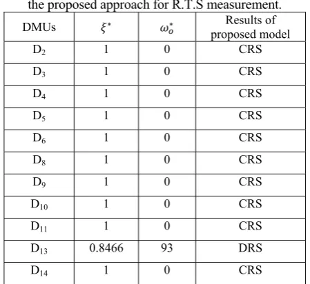
Table2. Table 2 represents the obtained results from the proposed approach for R.T.S measurement.

(9)

901

5. Conclusion

In this research, we first introduce a new input oriented model for determining efficient DMUs in the presence of Quasi-fixed inputs in regulated environment, then a new non-radial model is presented to estimate RTS of these DMUs in DEA.

Note that, since an inefficient DMU has more than one projection on the empirical function so, different returns to scales can be obtained for projections of the inefficient DMU by using the proposed RTS approach.

References

[1] Charnes, A., Cooper, W.W., Rhodes, E., 1978. Measuring the efficiency of decision making units. European Journal of Operational Research 2 (6), 429–444.

[2] Banker, R.D., Morey, R.C., 1986. The use of categorical variables in data envelopment analysis. Management Science 32, 1613–1627. [3] Cooper, W.W., Seiford, L.M., Tone, K., 2007. Data Envelopment Analysis: A Comprehensive Text with Models, Applications, References and DEA-Solver Software (Second Edition). New York, Springer Science+Business Media: Publisher. [4] Banker, R.D., 1984. Estimating most productive scale size using data envelopment analysis. European Journal of Operational Research 17 (1), 35–44.

[5] Banker, R. D., Charnes, A., Cooper, W. W. (1984). Some models for estimating technical and scale inefficiencies in data envelopment

analysis. Management Science, 30, 1078– 1092.

[6] Färe, R., Grosskopf, S. (1994). Estimation of returns to scale using data envelopment analysis: A comment. Journal of Operational Research, 79, 379–382.

[7] Ouellette , P. Quesnel , J-P. Vigeant, G. (2012). Measuring returns to scale in DEA models when the firm is regulated, European Journal of Operational Research .220 (2012) 571–576.

[8] Banker, R.D., Thrall, R.M., 1992. Estimation of returns to scale using data envelopment analysis. European Journal of Operational Research 62, 74–84.

[9] Charnes, A., Cooper, W. W., Golany, B., Seiford, L., Stutz, J. (1985). Foundation of data envelopment analysis for pareto-koopmans efficient empirical production functions. Journal of Econometrics, 30, 91–107.

[10] Khodabakhshi, M., Gholami, Y., Kheirollahi, H. (2010). An additive model approach for estimating returns to scale in imprecise data envelopment analysis. Applied Mathematical Modelling, 34, 1247–1257. [11] Ouellette, P., Vierstraete, V., 2004. Technological change and efficiency in the presence of quasi-fixed inputs: A DEA application to the hospital sector. European Journal of Operational Research 154, 755– 763.