Portfolio Performance Evaluation in a Modified Mean-Variance-Skewness Framework with Negative Data

409

Int. J. Data Envelopment Analysis (ISSN 2345-458X)

Vol.2, No.3, Year 2014 Article ID IJDEA-00231,13 pages

Research Article

Portfolio Performance Evaluation in a Modified

Mean-Variance-Skewness Framework with Negative

Data

Sh.Banihashemia*,M.Saneib, M.Azizia

(a) Department of Mathematics and Computer Science, Faculty of Econimics Allameh Tabataba’i

University.

(b) Department of Applied Mathematics, Islamic Azad University, Central Tehran Branch, Tehran,

Iran.

Received 28 May 2014, Revised 5 July 2014, Accepted 26 September 2014

Abstract

The present study is an attempt toward evaluating the performance of portfolios using variance-skewness model with negative data. Mean-variance non-linear framework and mean-variance-skewness non- linear framework had been proposed based on Data Envelopment Analysis, which the variance of the assets had been used as an input to the DEA and expected return and skewness were the output. Conventional DEA models assume non-negative values for inputs and outputs. However, we know that unlike return and skewness, variance is the only variable in the model that takes non-negative values. This paper focuses on the evaluation process of the portfolios in a mean-variance-skewness model with negative data. The problem consists of choosing an optimal set of assets in order to minimize the risk and maximize return and positive skewness. This method is illustrated by application in Iranian stock companies and extremely efficiencies are obtained via mean-variance-skewness non-linear framework with negative data for making the best portfolio. The finding could be used for constructing the best portfolio in stock companies, in various finance organization and public and private sector companies.

Keywords: Portfolio, Data Envelopment Analysis (DEA), Skewness, Efficiency, Negative data.

1. Introduction

In financial literature, a portfolio is an appropriate mix investments held by an institution or private

individuals. Evaluation of portfolio performance has created a large interest among employees also

academic researchers because of huge amount of money are being invested in financial markets. The

*_{Corresponding author: [email protected]. Tel:+98 21 22494937. Fax:+98 21 88524194.}

theory of mean – variance, Markowitz [11] is considered the basis of many current models and this

theory is widely used to select portfolios. This model is due to the nature of the variance in quadratic

form. . Due to quadratic form, a study by Arditti [1], Kane [9] and Ho and Cheung [7] shown that

investors prefer skewness which means that utility functions of investors are not quadratic. Other

problem in Markowitz model is that increasing the number of assets will be developed the covariance

matrix of asset returns and will be added to the content calculation. Due to these problems sharp one-

factor model is proposed by Sharp [16]. This method reduces the number of calculations required

information for the decision. Data envelopment analysis (DEA) has proved the efficiency for

assessing the relative efficiency of Decision Making Units (DMUs) that employing multiple inputs to

produce multiple outputs (Charnes et al [4]). Morey and Morey [13] proposed mean – variance

framework based on Data Envelopment Analysis, which the variance of the portfolios is used as an

input to the DEA and expected return is the output. Joro& Na [8] introduced mean - variance –

skewness framework and skewness of returns are also considered as an output. Briec et al. [3]

introduced shortage function. This shortage function obtains an efficiency measure that looks for

improvements in both mean and skewness and decreases in variance. Kerstence et al. [10] introduced

a geometric representation of the MVS frontier related to a new tool introduced in the literature by

Briec. Mhiri and prigent [12] analyze the portfolio optimization problem by introducing the higher

moments of the main financial index returns. In new models instead of estimating the whole efficient

frontier, only the projection points of the assets are calculated. In these models are used a non-linear

DEA-like framework where the correlation structure among the units is taken into account.

Conventional DEA models assume non-negative values for inputs and outputs. These models cannot

be used for the case in which DMUs include both negative and positive inputs and/or outputs. Poltera

et al. [14] consider a DEA model which can be applied in the cases where input/ output data take

positive and negative values.The other models solve negative data such as Modified slacks-based

measure model (MSBM) [2006], semi-oriented radial measure (SORM) [2010] and etc. The portfolio

optimization problem is a well-known problem in financial real world. The investor’s objective is to

get the maximum possible return on an investment with the minimum possible risk. Also the investors

prefer to maximize positive skewness. Since there are a large number of assets to invest in, this

objective leads to select the best assets via mean-variance-skewness non-linear model with negative

data.

The rest of the paper is organized as follows: Section 2 briefly reviews the portfolio performance

literature. Section 3 explainsmean-variance RDM and mean-variance-skewness RDM non-linear

models. Section 4 presents computational results using Iranian stock companies data and finally

2. Background

Portfolio theory to investing is published by Markowitz [11]. This approach starts by assuming that

an investor has a given sum of money to invest at the present time. This money will be invested for a

time as the investor’s holding period. The end of the holding period, the investor will sell all of the

assets that were bought at the beginning of the period and then either consume or reinvest. Since

portfolio is a collection of assets, it is better that to select an optimal portfolio from a set of possible

portfolios. Hence the investor should recognize the returns (and portfolio returns), expected (mean)

return and standard deviation of return. This means that the investor wants to both maximize expected

return and minimize uncertainty (risk). Rate of return (or simply the return) of the investor’s wealth

from the beginning to the end of the period is calculated as follows:

Return =(end−of−period wealth)—(beginning−of−period wealth)

beginning−of−period wealth (1)

Since Portfolio is a collection of assets, its return r_pcan be calculated in a similar manner. Thus

according to Markowitz, the investor should view the rate of return associated to any one of these

portfolios as what is called in statistics a random variable. These variables can be described expected

the return (min or r_p) and standard deviation of return. Expected return and deviation standard of

return are calculated as follows:

1/ 2

1 1 1

, (2)





 

  

 

 _  _

 



n



n n

p i i p i j ij

i i j

r r

Where:

n=the number of assets in the portfolio

p

r =The expected return of the portfolio

i

 =The proportion of the portfolio’s initial value invested in asset i

i

r =The expected return of asset i

p

 = The deviation standard of the portfolio

_ij= The covariance of the returns between asset i and asset j

In the above, optimal portfolio from the set of portfolios will be chosen that maximum expected return

for varying levels of risk and minimum risk for varying levels of expected return(Sharp [17] ).

Data Envelopment Analysis is a nonparametric method for evaluating the efficiency of systems with

concepts that will be used in other sections in DEA. They will not be discussed in details. Consider

j

DMU , ( j 1,...,n) where each DM U consumes m inputs to produce s outputs. Suppose that the

observed input and output vectors of DMU_j are X_j (x_1j, ...,x_mj) and Y_j (y_1j,...,y_sj) respectively, and let X _j 0and X _j 0, Y _j 0andY_j 0. A basic DEA formulation in input

orientation is as follows:

min ( )

1 1

. 1, ..., , (3)

1

1, ..., , 1

,

, 0,

0

 

 







     

  

   





   

     



s m

s s

r i

r i

n

s t x s x i m

j ij i io j

n

y s y r s

j rj r ro j

s s

Where



is a n-vector of



variables, sas-vector of output slacks,san m-vector of input slacks

and set is defined as follows:

with constant returns to scale,

with non-increasing returns to scale ,

with variable returns to scale

{

{ ,1 1}

{ ,1 1}

(4)

n R

n R

n R











 

 _ 

 _ 





  





Note that subscript ‘o’ refers to the unit under the evaluation. A DMU is efficient iff



1and all slack

variables s,sequal zero; otherwise it is inefficient (Charnes et al. [4]). In the DEA formulation

above, the left –hand sides in the constraints define an efficient portfolio. 𝜃 is a multiplier defines the

distance from the efficient frontier. The slack variables are used to ensure that the efficient point is

fully efficient. This model is used for asset selection. The portfolio performance evaluation literature

is vast. In recent years these models have been used to evaluate the portfolio efficiency. Also in the

Markowitz theory, it is required to characterize the whole efficient frontier but the proposed models

The distance between the asset and its projection which means the ratio between the variance of the

projection point and the variance of the asset is considered as an efficiency measure( )



. In this

framework, there is n assets,



_jis the weight of asset jin the projection point,

r

_jis the expected return of asset j,



_oand



_o2 are the expected return and variance of the asset under evaluation

respectively. Efficiency measure



can be solved via following model:

 

min ( )

1 2

. . ₁ ,

1 2 2 ( ( )) 2 1 1 0 1

5

                        

























s s n

s t E _{j j}r s _o j

n

E _j r_{j j} s _o

j n

j j

Model (5) is revealed by the non-parametric efficiency analysis Data Envelopment Analysis (DEA).

Joro and Na [8] extended the described approach in (5) into mean-variance-skewness framework

where



_ois the skewness of the asset under evaluation. The efficiency measure



can be solved

through using the following model:

 

min (_{1 2 3})

. . ,

1 1

2 2

( ( )) ₂

1 3 ( ( )) 3 1 1 0 1

6

                                 





































s s s

n

s t E _{j j}r s _o j

n

E _j r_{j j} s _o

j n

E _j r_{j j} s _o j

n j j

Model (6) projects the asset with the efficient frontier by fixing the expected return and skewness

Fig 1. Different projections (input oriented, output oriented, combinationoriented)

Fig 1 illustrates different projection that consist of input oriented, output oriented and combination

oriented in models of data envelopment analysis. C is the projection point obtained via fixing

expected return and minimizing variance, B via maximizing return and minimizing variance

simultaneously, and D via fixing variance and maximizing return.

In the conventional DEA models, each DMU_j(j1,..., )n is specified by a pair of non-negative

input and output vectors (x y_j, _j)Rm s , in which inputs x iij( 1,..., )m are utilized to produce

outputs, y_rj(r1,..., )s . These models cannot be used for the case in which DMUs include both

negative and positive inputs and/or outputs. Poltera et al.[14] consider a DEA model which can be

applied in the cases where input/ output data take positive and negative values. Rang Directional

Measure (RDM) model proposed by Polera et al. goes as follows:

1

1

1

max

1,..., ,

1,..., , (7)

1,

0 1,..., .



 

 











  

  



 







n

j ij io io

j

n

j rj ro ro

j

n

j j

j

st x x R i m

y y R r s

j n

Ideal point (I ) within the presence of negative data, is :

(max {_{j rj}: 1,..., }, min {_{j ij}: 1,..., }

I  y r s x i m where

0 5 10 15 20 25

0 50 100 150 200 250 300

Assets

Projection Points

D

A B B

,

min { : 1,..., }, 1,..., ,

max { : 1,..., } 1,..., . (8)

   

   

io io j ij

ro j rj ro

R x x j n i m

R y j n y r s

The other models solve negative data such as Modified slacks-based measure model (MSBM),

Emrouznejad [6], semi-oriented radial measure (SORM), Sharp et al. [15] and etc.

3. Modified models in the presence of negative data

In model (6) if return and skewness is considered positive then the results are correct, hence the

problem can happen only if return and skewness can take both positive and negative values. As we

know that unlike return and skewness, variance is only a non-negative number. Also, Bhattacharyya et

al. [2] predicted that for assets with negative expected returns, expected return will be a declining and

convex function of skewness. Assume the basic problem is to select a portfolio from n financial

assets. A portfolio



( ,...,



₁



_n)is a vector of proportions in each of these n financial assets with

n i i 1

1









. Excluding short sales, one must impose the condition



_i0for all i{1,..., n}. In general,

the set of admissible portfolio is written as follows:

n n

i i

i 1

{



R :



1,



0}



  



  .

Assets are characterized by an expected return E[r_i]. By a covariance matrixwith

ij cov(r , r )i j E[(ri E[r ])(ri j E[r ])]j (9)

    

And by a co-skewness tensor of rank three with:

ij E[(ri E[r ])(ri j E[r ])(rj k E[r ])]k (10)

     .

Then, we have:

n i i i 1

n 2

i j ij i, j 1 n 3

i j k ij i, j,k 1

E[r( )] E[r ]

V ar[r( )] E[(r( ) E[r( )]) ] (11)

Sk[r( )] E[(r( ) E[r( )]) ]











 







  









   

   







To condense notation, the function



: R3defined by: ( ) (E[r( )], V ar[r( )],Sk[r( )])

is introduced to represent the expected return, variance and skewness of a given portfolio



.In the

reminder, an element of R3is called a MVS point. Thus, a MVS point can be the image by of a

portfolio, or any arbitrary point in this three-dimensional space. It is useful to define the MVS image

of as the image



( ) , with

( ) { ( ); }.



 

  

 

This set can be extended by defining a MVS disposal representation set via:

DR   



( ) (R_R_R )._

For the purpose of gauging portfolio efficiency, a subset of this representation set the weakly and

strongly efficient frontier must be defined as:

Definition 1: In the MVS space, the weakly efficient frontier is defined as:

w ' ' ' ' ' '

( ) {(M, V, S) DR; ( M , V , S ) ( M, V, S) (M , V , S ) DR}

           .

Definition 2: In the MVS space, the strongly efficient frontier, is defined as:

s ' ' ' ' ' ' ' ' '

( ) {(M, V, S) DR; ( M , V , S ) ( M, V, S)and ( M , V , S ) ( M, V, S) (M , V , S ) DR}

               

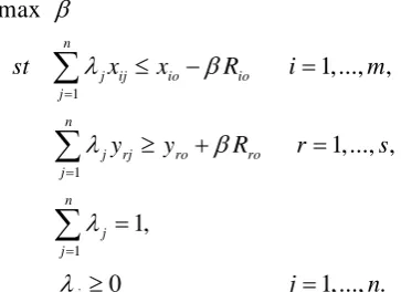
Extremely, we present following non-linear mean-variance RDM model on the basis of negative data:

2 o

n

j j o o

j 1 n

2 2

j j j o

j 1 n

j j 1

max

s.t. E r R

E ( (r )) R (12)

1 0                                  







Ideal point (I ) within the presence of negative data, is

2 o

2

j j j j

o j j o

2 2

o j j

I (min { }, max { }) where,

R max { : j 1,..., n} (13)

R min { : j 1,..., n}.

 













      

The above model can be expressed as following:









2

o o o 2 o n j j 1 max

s.t. E r( ) R

Var r( ) R (14)

Also, we present following non-linear mean-variance-skewness RDM model on the basis of negative data: 2 1 2 2 1 3 1 1 max . . ( (15) ( ) 1 0                              _{ }  _  _   _{ }    _{ }  _  _   _{ }     









o o o n

j j o

j

n

j j j o

j

n

j j j o

j

n

j j

j

s t E r R

E r R

E r R

Ideal point (I ) within the presence of negative data, is

2

j j j j j

I(min {



}, max {

 

, })

Where

 

 

 

o 2 o o j o 2 2 o o j o R max

R min (16)

R max   













     

The above model can be expressed as following:













2 2 1 max . . ( )

( ) (17)

( ) 1 0                        



o o o o o o n j j j

s t E r R

Var r R

Sk r R

The methodology in this paper starts with asset selection via performance evaluation in presence of

negative data. The data used for this methodology is from 20 Iranian stock companies. In many cases

similar to this example there are a lot of assets. It is better that starts with asset selection via

performance evaluation. The choice of the asset can be random or discrete. The random choice of

assets is usually biased and do not promise an optimum portfolio; hence it is more rational to have an

objective choice while selecting the assets to be included in the portfolio. Performance evaluation is

calculated by using models 14 and 17.

4. Application in Iranian Stock Companies

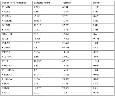
We illustrate our approach in non-linear mean-variance-skewness model for a data set 20 Iranian

stock companies. A list of stocks used is provided in Table 1. In this report, there is expected return,

variance, skewness of stocks which expected return and skewness are considered as output and

variance is as input. The example is received from Iranian stock companies and is about portfolio

performance evaluation in a mean-variance-skewness RDM framework. Thus, we know that unlike

return and skewness, variance is the only variable in the model that takes non-negative values. In the

analysis, the variance of the stocks is used as an input to the DEA and expected return and skewness

are used as output.

Table1. Descriptive statistics of the Iranian stock companies

Iranian stock companies Expected return Variance Skewness

VNVIN 7.285 6.534 -1.503

VPARS 7.388 10.474 0.789

VBHMN -2.193 3.720 -0.470

VPASAR 10.853 4.256 0.813

DGABR 12.517 32.259 0.540

STRAN 9.052 70.764 1.488

FBAHNR 52.511 57.497 -0.6

FMLI -3.676 19.609 -0.851

FVLAD 3.537 21.496 -1.03

KCHINI 7.57 67.378 0.591

VTVSA 6.896 14.171 -0.270

VLSAPA 1.888 29.002 -.964

VNFT 18.737 42.133 -1.314

VTGART 1.302 12.419 -0.947

VKHARZM 1.231 1.611 -1.048

VSAKHT 14.741 11.429 -0.922

KHSAPA 3.896 25.358 -0.853

VSINA 2.967 4.856 0.499

RTKG 32.677 28.464 0.487

VBMLT 2.022 1.56 -0.589

Linear MV and linear MVS with RDM model are calculated at table 2. Also, non linear MV

efficiency measure and non-linear MVS efficiency measure using models 14 and 17 are calculated at

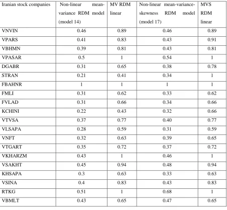
Table2. Efficiency measure of the Iranian stock companies Iranian stock companies Non-linear

mean-variance RDM model (model 14)

MV RDM linear

Non-linear mean-variance-skewness RDM model (model 17)

MVS RDM linear

VNVIN 0.46 0.89 0.46 0.89

VPARS 0.41 0.83 0.43 0.91

VBHMN 0.39 0.81 0.43 0.81

VPASAR 0.5 1 0.54 1

DGABR 0.31 0.65 0.38 0.78

STRAN 0.21 0.41 0.34 1

FBAHNR 1 1 1 1

FMLI 0.31 0.62 0.33 0.62

FVLAD 0.31 0.66 0.34 0.66

KCHINI 0.22 0.43 0.32 0.66

VTVSA 0.37 0.77 0.40 0.77

VLSAPA 0.28 0.59 0.31 0.59

VNFT 0.32 0.63 0.39 0.65

VTGART 0.35 0.72 0.37 0.72

VKHARZM 0.43 1 0.46 1

VSAKHT 0.45 0.94 0.48 0.94

KHSAPA 0.3 0.63 0.33 0.63

VSINA 0.4 0.83 0.43 0.83

RTKG 0.51 1 0.68 1

VBMLT 0.43 0.65 0.47 0.65

Table 2 represents the calculated and compared the results of efficiency of model 14 and model 17 to

linear MV RDM model and linear MVS RDM model. As seen in Table 2, model 14 and model 17

scores are as a conservative estimate of the linear MV RDM and linear MVS RDM scores. In this

example all the linear DEA scores are greater than the non-linear model.Also, we compare the results

linear MV RDM and linear MVS RDM. Because of, skewness equation is increased the results are not

better. But, we know that the RDM model gives inefficiency score. Therefore, the efficiency score

linear MVS RDM model is greater than linear MV RDM. But, those having positive skewness, have

more efficiency increasing. For example, STRAN having the most positive skewness, Firstly linear

MV RDM efficiency score has 0.41 and linear MVS RDM efficiency score ,secondly becomes 1. But

scores are become nearly better than non-linear MV RDM efficiency scores. But those having positive

skewness, have more efficiency increasing. For example, STRAN and KCHINE.

The results are obtained by General Algebraic Modeling System (GAMS) software.

5. Conclusion

This paper introduced a measure for portfolio performance using non-linear

mean-variance-skewness RDM model. Joro and Na had proposed models for evaluating portfolio efficiency in which

Data Envelopment Analysis model was employed. In these models was used a non-linear DEA-like

framework where the correlation structure among the units was taken into account. We have applied

model 14, and model 17 with return and skewness as output and the variance as the input to 20 stocks.

The detailed results are presented in Table 2. In the numerical example is also observed that

compared with linear, these models are highly exact in all the units, that is, all the linear DEA scores

are greater than the non-linear models. This means that the DEA frontier is always dominated via the

non-linear modified mean-variance frontier. But, those having positive skewness, have more

efficiency increasing. For example, STRAN having the most positive skewnes. Firstly, linear MV

RDM efficiency score has 0.41 and linear MVS RDM efficiency score, Secondly becomes 1. But

those having negative skewness, don’t change in efficiency score. Non-linear MVS RDM efficiency

scores are nearly better than non-linear MV RDM efficiency scores. But, those having positive

skewness, have more efficiency increasing. For example, STRAN and KCHINE.

Acknowledgement

The authors’ sincere thanks go to the known and unknown friends and reviewers who meticulously

covered the article and provided us with valuable insights.

Reference

[1] Arditti, “Skewness and investors_ decisions: A reply,” Journal of Financial and Quantitative

Analysis, vol. 10, pp. 173–176, 1975.

[2] Na. Bhattacharyya, Th. garrett, St. Louis, “Why people choose negative expected return assets- an

emprical examination of a utility Theoretic explanation ,2006.

[3] W. Briec, K. Kerstens and O. Jokung, “Mean-Variance-Skewness Portfolio Performance Gauging:

A General Shortage Function and Dual Approach,” Management Science, vol. 53,pp 135 – 149, 2007. [4] A. Charnes, W.W. Cooper and E. Rhodes, “Measuring Efficiency of Decision Making Units,”

[5] A. Charnes, W.W. Cooper and Lewin, A.Y. Seiford, “Data Envelopment Analysis: Theory, Methodology and Applications,”Kluwer Academic Publishers, Boston, 1994.

[6] A. Emrouznejad,, “A semi-oriented radial measure for measuring the efficiency of decision

making units with negative data, using DEA”, European journal of Operational Research, 200,pp.

297-304, 2010.

[7] Y.K.. Ho and Y.L. Cheung, “Behavior of intra-daily stock return on an Asian emerging market— Hong Kong,” Applied Economics, vol. 23, pp. 957–966, 1991.

[8] T. Joro and P. Na, “Portfolio performance evaluation in a mean-variance-skewness framework”

European Journal of Operational Research, vol. 175,pp. 446–461, 2005.

[9] A. Kane, “Skewness preference and portfolio choice,” Journal of Financial and Quantitative

Analysis, vol. 17, pp. 15–25, 1982.

[10] K. Kerstens, A. Mounir and I. Woestyne, “Geometric representation of the

mean-variance-skewness portfolio frontier based upon the shortage function, European Journal of Operational

Research, pp. 1-33, 2011.

[11] H.M. Markowitz, “Portfolio selection,” Journal of Finance, vol. 7, pp. 77–91, 1952.

[12] M. Mhiri and J. Prigent, “International portfolio optimization with higher moments,”

International Journal of Economics and Finance, Vol. 2, no. 5, pp. 157-169, 2010.

[13] M.R. Morey and R.C. Morey, “Mutual fund performance appraisals: A multi-horizon perspective with endogenous benchmarking,” Omega, vol. 27,pp 241–258, 1999.

[14] M.C. Portela, e. Thanassoulis, and g. Simpson, “A directional distance approach to deal with

negative data in DEA : An application to bank branches, ”Journal of Operational Research Society,

55 ,pp. 1111-1121, 2004.

[15] JA. Sharp, W. Meng and W. Liu, “A modified slacks-based measure model for data envelopment

analysis with ‘natural’ negative outputs and inputs, “ Journal of the Operational Reaserch Society, 57,

pp.1-6, 2006.

[16] W.F. Sharpe, “Capital asset prices: A theory of market equilibrium under conditions of risk,”

Journal of Finance, vol. 19,pp. 425–442, 1964.