Modelling of stationary three-dimensional separated air flows around an Ahmed reference model

Modelling of Stationary Three-Dimensional

Separated Air Flows around

an Ahmed Reference Model

P. Gilliéron,

Renault S.A.; 1 Avenue du Golf, 78288 Guyancourt Cedex e-mail: [email protected]

F. Chometon,

Conservatoire National des Arts et Métiers, 15, rue Marat, 78210 Saint Cyr l’Ecole e-mail: [email protected]

Abstract: When analysing the topology of turbulent flow systems for alternative vehicle configurations, conventional wind-tunnel tests may not be sufficient. Vehicle development teams investigating this kind of physical phenomenon are increasingly interested in numerical simulation, but reliable implementation of computational techniques in automotive aerodynamics requires validation to confirm that such methods are capable of accurately reproducing experimentally proven physical behaviour. We address this issue by comparing the results of experimental wind-tunnel tests with simulated values for aerodynamic drag coefficient and vortex wake flows at different angles of car rear window inclination, using an Ahmed [1] reference model.

1 - INTRODUCTION

To meet targets for shorter lead-times and lower costs in modern automobile design processes, aerodynamics specialists are constantly seeking new solutions capable of providing prompt and accurate guidance in design practice. One such solution is numerical simulation, which provides a valuable complement to results obtained from experimental wind tunnel tests. However, if computational techniques are to become a viable proposition in automotive aerodynamics, they must demonstrate their ability to accurately reproduce the elementary phenomena observed on simple geometric forms in the wind tunnel. With this objective in mind, we discuss computational work on an Ahmed reference model (Ahmed, Ramm and Faltin, 1984 [1]), following the work of Baxendale, Graysmith, Howell and Haynes (1994 [2]). The Ahmed model was chosen for its geometrical simplicity, and because of the body of documented experimental results available for this model in automotive aerodynamics applications. Specifically, we compare computed results against experimental findings for different angles of rear window inclination, and offer qualitative analysis, chiefly concerning aerodynamic drag coefficient and the behaviour of vortex wake flows.

2 - EXPERIMENTAL RESULTS

The Ahmed reference model is shown in figure 1. The angle α represents the angle of inclination of the rear window with respect to the horizontal.

Fig. 1 - Ahmed Reference Model

taken in the Göttingen open-section wind tunnel (Ahmed et al [1]). The Reynolds number was 4 106, the initial flow turbulence index was 0.5%, and the total model length was around 1 m. Results revealed two basic airflow patterns, delimited by upper and lower threshold values α_me and α_Me for the angle of inclination α. Ahmed's values for these

critical angles α_me and α_Me were 12 and 30 degrees respectively. Wake flow is

two-dimensional for values of α below α_me , then becomes three-dimensional between α_me and

α_Me _{, then reverts to two-dimensional behaviour for values of α above α} M e _.

i) Two-dimensional base flow : 0≤ α < αme - For rear window inclinations below αme ,

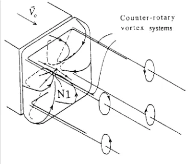
the flow from over the roof remains tangential to the rear window and separates over the whole of the base area (see a and b in figure 2). Two parallel sets of flows (from the roof and floor and from the two side walls) set up two counter-rotary vortex flows, which together form a toroidal vortex system exercising pressure on the base (see figure 3). Then further downstream, this toroid flow dissipates in the wake (Huchot, 1990 [3]).

Fig. 2 – Ahmed’s wake flow behaviour [1]

Fig. 3 – Wake separation, see [1].

At the base surface, the converging toroid streamlines generate a singular point in the form of an attachment node, identified as N1 in figure 3. The location of this point is directly governed by the intensities of the vortex flow systems from the floor and roof, and varies with the exterior velocity around the base (Chometon, 1985 [4]). As α increases from 0 to

α_me

, the rear window flow remains attached to the wall but experiences a downward inflection, and the attachment point N1 moves down.

(ii) Three-dimensional hatchback flow : α_me ≤ α ≤ α_Me - As α rises above the lower critical angle α_me (see c in figure 2), the flow suddenly starts to display highly three-dimensional behaviour around the rear window. The vortex wake system takes the form of two counter-rotary lateral vortices (T) starting at a separation line AB, and we observe an open separation bulb, D, located at the upper part of the rear window (see figure 4 and c on figure 2). The fluid inside the separation bulb experiences a rotary motion (centred around point A) that generates two singular points, S1 and S2. The base flow combines with the rear window flow to generate a detachment node N2 (see figure 4).

0,15 0,20 0,25 0,30 0,35 0,40

0 10 12 20 25 30 40 50

A ngles (degrees) Cd

α_Me

αe_m

Fig. 4 – Ahmed’s wake flow behaviour [1], Fig. 5 – Ahmed’s aerodynamic drag, [1] schematic view.

2.2 – AERODYNAMIC DRAG COEFFICIENT - For α values from 0 to α_me , aerodynamic drag, solely governed by the dimensions of the separated area around the base, decreases with the inclination (Onorato, Costelli and Garonne, 1984 [5]). Then as α rises above the lower critical angle α_me , a separation bulb forms. Because this absorbs a growing amount of energy, we observe an increase in aerodynamic drag. But as α rises still further, above the upper critical angle α_Me , airflow no longer feeds the vortex systems associated with the separation bulb, and these systems therefore dissipate in the wake (Chometon and Gilliéron, 1996 [6]). Static and total pressures in the base area experience a sudden rise, and the aerodynamic drag drops. The drag value is governed by the area of the base zone, and is close to that measured for zero rear window inclination (see figure 5).

3 - COMPUTED RESULTS

The triangular surface meshing used for computation purposes was obtained using version 7.2 of the Ansa software. For each computation configuration, the Ahmed reference model was represented by a total of around 15,000 triangular surface elements.

For areas not experiencing separation phenomena, nodes were spaced at intervals of 2 10-2 m, which represents 2 10-2 times the length of the body and is of the same order of magnitude as the thickness of the boundary layer prior to separation. In the zones that do experience separation (especially around the rear window and base) the spacing is four times closer, at 5 10-3 m. Computation is performed for a half-vehicle in the y-positive half-space. If L is the vehicle length, the fluid section is represented by a rectangular parallelepiped of height 2L, width 2L and length 8L. The fluid section is 2L high at the front of the body and 5L high at the rear. These dimensions allow infinite-atmosphere flow modelling.

ESAIM PROC VOL 7 1999 176 182

Outside this region, tetrahedral volume meshing was applied using the Fluent package’s automatic "Init and Refine" procedure. Across all geometrical configurations, the model had a total of around 300,000 prism and tetrahedron volume cells.

Computation was performed using version 4.2 of the Fluent software, assuming stationary flow and incompressible fluid conditions, and an uniform inlet velocity of 60 m/s. For a characteristic infinite airflow upstream length of half the fluid section height and a non-perturbed turbulence rate of 0.5%, the mixing length was 5 10−3 m. A k− ε model was used, with a logarithmic law of the wall. At the fluid section outlet, a constant pressure condition was applied. For each solution, 300 first-order iterations were performed, followed by 800 second-order iterations. Classical numerical schemes were used, and default relaxation values were taken for the continuity and momentum equations.

The volume meshing was then adapted on the basis of static pressure gradients to obtain a quasi-continuous pressure field covering the whole of the computation domain. This adaptation was performed by successive iterations on a hundredth of the total number of cells representing the fluid domain, monitoring the impact of adaptation by observing the value of aerodynamic drag, which decreases with the pressure gradient. After adaptation, we had a total of around 450,000 volume cells.

For different configurations, numerical experimentation was performed by varying the angle of inclination of the rear window, α, from 0 to 50 degrees from the roof horizontal. In the cases outlined below, friction lines or wall stresses were computed from the velocity determined at the centre of the prisms adjacent to the body walls.

3.1 – AERODYNAMIC DRAG COEFFICIENT - Figure 6 shows a comparison

between computed and experimental values for aerodynamic drag coefficient (Cd).

Computed values of aerodynamic drag coefficient are higher than experimental values but show the same basic pattern for variations in rear window angle. The best correlation is found around the critical angle α_Me = 30 degrees.

0,20 0,25 0,30 0,35 0,40

0 10 12 20 25 30 40 50

A ngles (degrees) Cd

αcm

αc M

αe_m

αe M

Experimental Computed

3.2 – AIRFLOW SYSTEMS - Computed results reveal two airflow patterns, delimited by

the upper and lower threshold angles α_me and α_Me

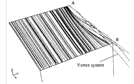
i) Two-dimensional base flow : 0≤ α < α_me - For the rear window inclination up to α_me , analysis of streamlines in the volume close to the rear window shows that the airstream from the roof remains tangential to the rear window (see figure 7). Then as α increases, the friction lines start to curve toward to the outer edge, AB, of the rear window, with lateral vortices forming at around 10°.

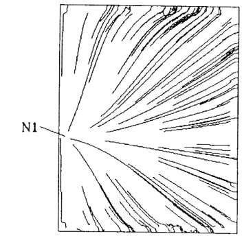
Figure 8 shows air feed to the resulting vortex cone, which diffuses and dissipates in the wake. Around the base, streamlines from peripheral separation generate a toroid vortex system (see figure 7). The plot of friction lines on the base surface (figure 9) clearly shows the node point N1, which moves down as the rear window angle, α, increases.

Outside a small area located at the top of the rear window, computed values for static pressure coefficients on the rear window and base correlate well with experimentally observed values. For example, at α = 12°, computed static pressure coefficients range from -0.05 to -0.15, compared to Ahmed’s value of -0.15.

Fig. 7 – Sreamlines over roof, for α = 10°.

Only half body is represented. Fig. 8 – Friction lines on rear window, for _{Only half body is represented.} α = 10°.

On the rear window, computed static pressure coefficients range from -0.15 to -0.65, compared to Ahmed’s values from -0.15 to -0.50 (see figure 10). Computation is also accurate in predicting the static pressure distribution typical of a vortex shedding along AB. The over predicted computed drag values (figure 6) can probably be explained by the code’s tendency to overestimate pressure drop at the base. This shortcoming might by related to defective simulation of wake vorticity, in turn arising from defective simulation of the boundary layer.

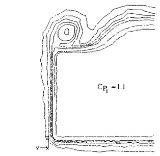
In the wake around the base computed tomographies for total pressure loss match the experimentally observed values with experimentally observed structures for this kind of object (see figure 11). The distribution of total pressure coefficients, from 0 to 1.2, is classic.

Distribution and order of magnitude of static pressure coefficients and total pressure losses around the base are also consistent.

Fig. 9 – Friction lines on base, for α = 10°. Only half body is represented.

Fig. 10 – Computed pressure coefficients (left) and experimental pressure coefficients (right), for α = 12°. Lengths on the left-hand plot are not significant.

Fig. 11 – Total pressure tomographies for α = 10°, at X = X base + 0.010 m

Fig. 12 – Velocity field at X = X base + L/2, where L is length of Ahmed model for α = 10°.

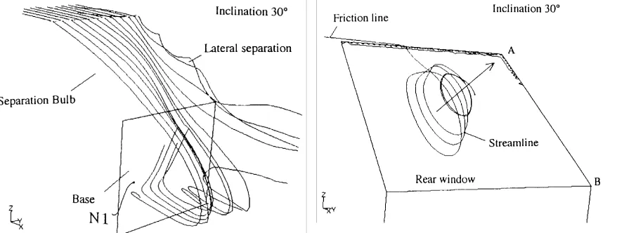
ii) Three-dimensional “hatchback” flow : α_me ≤ α ≤ α_Me - As α rises from the lower critical angle α_me to the upper critical angle α_Me , a separation bulb develops at the top of the rear window. At the lower part of the rear window we observe streamlines feeding lateral separation and base vortices (see figure 13).

The flow starts to separate at the boundary between the roof and the rear window. Inside the bulb, streamlines are fed by a rotary motion. Some streamlines form a spiral generating a system of friction lines centred around point A (see figure 14). This topology appears clearly on Ahmed’s [1] parietal visualization (see figure 4). Figure 4 should be compared with figure 16, on which the bulb outline has been drawn in by hand.

the vortex shedding, suggests the existence of a separation focus, F, which would in turn imply that the separation bulb was open. The attachment node N2 and the focus F appears clearly in figure 16 but not in Ahmed’s parietal visualization or in figure 4, see also [1].

From a topological point of view, there is a saddle point associated with each pair formed by an attachment node and a separation focus (Chometon and Gilliéron, 1994 [7]).This saddle point is marked S3 on figure 16. By symmetry, the whole set of nodes and foci will generate two saddle points, S1 and S2 in the plane of symmetry Y=0 (figures 16, 17 and 4).

Fig. 13 – Separation bulb at α = 30°. Only half body is represented.

Fig. 14 – Streamlines on rear window, at α = 30°. Only half body is represented.

On the rear window, friction lines come under the influence either of the separation focus or of the lateral separation line, AB (see figure 17), depending on their location. Sreamlines close to the separation bulb are curved in the direction of rotation set up by focus F, to generate the saddle point S2. Streamlines close to the rear window separation line AB curve outward and the local flow feeds the vortex cone forming at this separation line. Some friction lines converge laterally at the lower part of the rear window to feed a singular point in the form of a separation node at N3.

Fig. 15 – Interaction between separation bulb and base vortex, at α = 30°. Only half body is represented.

Fig. 16 – Friction lines on rear window, attachment node N2, separation focus F and saddle point S3, at α = 30°. Only half body is represented.

the base a toroidal system that exercises pressure on the base and develops along two counter-rotary vortices.

Except in an area located at the centre of the base, computed static pressure coefficients (from -0.05 to -0.20) are of the same order of magnitude as experimental values. Away from the junction with the base, the distribution and values for static pressure coefficients on the rear window (from -0.25 to -0.75) correlate well with Ahmed’s values (see figure 18).

Fig. 17 – Friction lines on rear window, saddle pointS1 and S2, separation node N3, at α = 30°. Only half body is represented.

Fig. 18 – Computed pressure coefficients (left) and experimental pressure coefficients (right), for α = 30°. Lengths on the left-hand plot are not significant.

Computed tomographies for total pressure loss in the wake at 0.010 m downstream of the base (figure 19) show structures and values that correlate well with experimentally observed results on this kind of object (Chometon and Laurent, 1985 [9]). This plot also confirms the open nature of the separation bulb.

Fig. 19 – Cut-off pressure tomographies at

0.010 m downstream of base for α = 30°. Fig. 20 – Numerical wall display for a = 40°. Only half_{body is represented.}

iii) Two-dimensional base flow : α > α_Me - As α rises above the upper critical angle

α_Me

, the friction lines on the rear window revert from a three-dimensional to a two-dimensional pattern, the final form of which (as shown in figure 20) is typical of a base flow (α =_{90 degrees). Of all the singular points observed between the two critical angles,} only the node N1 remains.

4 - CONCLUSIONS

Computed results obtained on the Ahmed reference model using version 4.2 of the Fluent software are in agreement with experimental results obtained in the wind tunnel. In particular, computation successfully reproduces changes in vortex wake airflows and aerodynamic drag coefficients during transitions from two-dimensional base behaviour to three-dimensional hatchback behaviour and back again. And computed values for the critical angles at which these transitions occur correlate well with experimental findings.

Computed results suggest that the flow topology associated with the separation bulb on the rear window corresponds to a classic hatchback configuration, and that it varies continuously around the angle αm.

Our results show numerical simulation to be a highly promising technique for investigating physical phenomena in automotive aerodynamics. From the good results obtained on the simple shapes of an Ahmed reference model, it would clearly appear viable to integrate computational methods in the analysis phases of a vehicle development cycle, since the friction line topologies for an Ahmed reference model are identical to those observed on an actual vehicle.

By accurately revealing the processes involved in the formation and development of elementary three-dimensional separated flows, numerical modelling can be of valuable assistance to design personnel seeking to understanding this kind of physical phenomenon. Computational methods thus look set to play a vital role in vehicle development work, alongside experimental wind tunnel tests.

REFERENCES

[1] AHMED S.R., RAMM R. and FALTIN G.; Some salient features of the time-averaged ground vehicle wake SAE technical Paper Series 840300, Detroit 1984. [2] BAXENDALE A.J., GRAYSMITH J.L, HOWELL J.P. and HAINES T.;

Comparisons between CFD and experimental results for the Ahmed reference model; RAeS Conference on Vehicle Aerodynamics, pp 30.1-30.11, 1994.

[3] HUCHOT W. H.; Aerodynamics of road vehicle, From fluid mechanics to vehicle engineering, Flow field around a passenger car, pp 110-115, 1990.

[4] CHOMETON F.; Analysis of three-dimensional separated flow on bluff bodies, Second IAVD congress on Vehicle Design and components, Geneva, 4-6 March 1985.

[5] ONORATO M., COSTELLI A. and GARONNE A.; Drag measurement through wake analysis, SAE, SP-569, International Congress and Exposition, Detroit, Michigan, 27 February – 2 March, pp 85-93, 1984.

[6] CHOMETON F. and GILLIÉRON P.; A survey of improved techniques for analysis of three-dimensional separated flows in automotive aerodynamics, SAE Congress, Detroit, Michigan, 27-29 February 1996.

[7] CHOMETON F. and GILLIÉRON P.; Dépouillement assisté par ordinateur des visualisations pariétales en aérodynamique, Compte-rendu Académie des Sciences Paris, série II, pages 1149-1156, 1994.

September 25-30, vol II, pp 2.364-2.371, 1988.