J.-S. Dhersin, Editor
TIME-IMPLICIT HYDRODYNAMICS FOR EULER FLOWS
∗Serge Van Criekingen
1, Edouard Audit
1, Jeaniffer Vides
2and Benjamin
Braconnier
3Abstract. We consider the Euler equations with gravity source terms, and derive a time-implicit resolution scheme from the explicit one developed by Vides et al. [8]. This requires computing a Jacobian matrix, which is done symbolically using the automatic differentiation tool TAPENADE developed at Inria. The resulting sparse linear system is solved using thePETSclibrary. We present parallel numerical results for a 2-D Rayleigh-Taylor instability on up to 4096CPU cores.
R´esum´e. Nous consid´erons les ´equations d’Euler avec des termes sources d´ecrivant la gravitation, et nous construisons un sch´ema de r´esolution implicite en temps sur base de celui, explicite, d´evelopp´e par Vides et al. [8]. Le calcul d’une matrice jacobienne est requis, et il est r´ealis´e symboliquement en utilisant l’outil de diff´erentiation automatique TAPENADE developp´e `a Inria. Le syst`eme lin´eaire obtenu est r´esolu via la biblioth`eque parall`elePETSc. Nous pr´esentons des r´esultats num´eriques pour l’instabilit´e de Rayleigh-Taylor en deux dimensions, obtenus en utilisant jusqu’`a 4096 cœursCPUen parall`ele.
Introduction
The starting point of this study is the explicit scheme developed by Vides et al. [8] for the Euler-Poisson model, i.e., the Euler equations supplemented by gravitational effects. This development was done in view of numerically simulating gravitational flows in astrophysics, and implemented within the HERACLES [4, 7] astrophysics code. The scheme in [8] is based on a finite volume discretization with a Godunov-type solver for the Euler equations, and a finite difference discretization with standard Krylov-type solver for the Poisson equation. The specificity of this scheme is that the Godunov-type solver for the Euler equations takes into account the gravitational effects. Moreover, it uses a relaxation procedure for the thermodynamic pressure and the gravitational potential.
We here aim at developing an implicit version of the explicit scheme developed by Vides et al. However, in this first study, we do not consider the full Euler-Poisson model, but rather focus on the Euler equations with gravity source terms. The interest of developing an implicit scheme is to overcome the restriction due to the CFL condition. This condition can be very restrictive in systems in gravitational equilibrium, e.g. stars, where movements are typically very slow. Similarly to [8], our developments are made within theHERACLES [4, 7] code.
∗The authors wish to thank Mikolaj Szydlarski for fruitful discussions.
1 CEA, Maison de la Simulation, USR 3441, CEA - CNRS - INRIA - Univ. Paris Sud - UVSQ, Gif-sur-Yvette, France 2 INRIA, Maison de la Simulation, USR 3441, CEA - CNRS - INRIA - Univ. Paris Sud - UVSQ, Gif-sur-Yvette, France 3 IFP Energies Nouvelles, Rueil-Malmaison, France
c
EDP Sciences, SMAI 2014
In our study, the Jacobian matrix, inherent to any implicit scheme, is computed symbolically by automatic differentiation using theTAPENADEcode [5, 6]. As for the resulting linear system, it is solved usingPETSc, a suite of data structures and routines for the scalable parallel solution of scientific applications modeled by partial differential equations, which has been used in many large-scale application projects [1–3].
The paper is organized as follows. In Section 1, the Euler equations with gravity source terms are introduced, as well as most of our notations. Then, Section 2 briefly describes the explicit setting of the scheme in [8] for which we propose an implicit version, described in Section 3. Numerical results are presented in Section 4, for a classical Rayleigh-Taylor instability test case in two dimensions. Note that we here do not perform a full performance comparison between the implicit and explicit schemes. As explained in Section 4, such a comparison would be fair only given a clear target result of interest, which is not the case in this general presentation of first implicit results. However, we investigate the weak and strong scalability of both explicit and implicit schemes on up to 4096 CPUcores.
1.
Mathematical Model
The Euler equations with gravity source terms can be written as
∂tρ + ∇ ·(ρu) = 0
∂tρu + ∇ ·(ρu⊗u+p) = −ρ∇φ
∂tρE + ∇ ·((ρE+p)u) = −ρu· ∇φ
(1)
where ρ > 0 is the density, u∈Rd the velocity (with dthe space dimension), E the specific energy and φ a
smooth gravity potential. The thermodynamic pressure pis modeled as a function of the density ρ and the internal specific energy = E− |u|2/2. The pressure law can typically be the perfect gas equation of state p(ρ, ) = (γ−1)ρwithγ a given constant.
For notational simplicity, we group the hydrodynamic unknowns into the state vector W = (ρ, ρu, ρE)T, such as to rewrite (1) as
∂tW+∇ ·F(W) +B(W)∇φ= 0, (2)
where
F(W) = ρu, ρu⊗u+p,(ρE+p)uT, B(W) =ρ(0d,e1, ...,ed,u)
T
,
(3)
with0d andei being respectively the null and ith canonical vector inRd.
Lastly, the admissible state vectors form the convex set Ωd:
Ωd= (
W∈R2+d; ρ >0, u∈Rd, E−|u|
2
2 >0
)
. (4)
2.
Reminder of the Explicit Scheme
In [8], the Euler equations with gravity (1) are handled with a finite volume discretization and a Godunov-type solver which takes into account the gravitational effects. For notational simplicity, we here adopt a 1-D setting. Assuming a uniform mesh with cells of size ∆x, the state vector in the mesh cell of indexievolves from timetn to timetn+1=tn+ ∆tas
Wni+1=Win−
∆t
∆x
FL,ni+1 2
−FR,ni−1 2
(5)
where FL,ni+1 2
and FR,n
i−1 2
are the left and right numerical fluxes, as in the traditional finite volume framework.
These numerical fluxes are obtained by solving Riemann problems at the cell interface xi±1
2, such thatF
depends onWn
i andWin+1, andF
L,n i−1 2
depends onWn
i andWni−1. Note that the discretized gravity source term
is introduced into the approximate Riemann solver, as described in [8]. Note furthermore that the resulting numerical fluxes are not conservative (i.e.,FL,n
i±1 2
6
=FR,n
i±1 2
) due to the gravity term.
3.
Implicit Scheme
Formally, changing from an explicit to an implicit scheme consists only in considering the fluxes on the right-hand side of (5) at time stepn+ 1 instead ofn:
Win+1=Wni − ∆t
∆x
FL,ni+1+1 2
−FR,n+1
i−1 2
. (6)
We follow a linearly implicit approach leading to a Jacobian linear system, as we now describe. First we define
Fi=
1 ∆x
FL,ni+1+1
2
−FR,ni−1+1 2
.
Note that, through the Riemann solvers, Fi can be seen as a function of the state vector values at time step
n+ 1 such that from equation (6) we may write
Win+1−Wn i
∆t =−Fi(W
n+1
i ,W n+1
i±1)
for each mesh cell i. The equivalent for the whole mesh of this last expression reads
Wn+1−Wn
∆t =−F
Wn+1.
where F is the global equivalent to Fi, including the appropriate boundary conditions. A first-order Taylor
approximation applied toF then yields
Wn+1−Wn
∆t ≈ −F(W
n)− ∂F
∂W
Wn+1−Wn
where ∂∂FW is the Jacobian matrix. We then have
J Wn+1−Wn≈ −F(Wn) (7) whereJ is defined as
J = I ∆t +
∂F ∂W
withI the identity operator. Note thatJ is not symmetric, but block symmetry is achieved.
4.
Numerical Tests
4.1.
Benchmark Presentation
We consider the Rayleigh-Taylor instability in 2-D. This instability consists in the fall of a dense fluid into a lighter one due to gravitation. Initially, both fluids are totally segregated, with the dense one on top. We here consider a 2-D model of this experiment, in thex−yplane, with gravity acting opposite to thex-direction. The computational domain is (0, Lx)×(0, Ly) withLx= 4m,Ly = 1m, and the uniform gravity potential is given
byφ=g xwithg= (−10,0)m.s−2. At timet= 0, the interface between the two fluids is perturbed as follows:
the dense fluid fills all the points in the domain for which x > 1 2Lx
1− 1 10cos((
y Ly −
1 2)π)
. Both fluids are
assumed to be governed by a perfect gas equation of state: p = (γ−1)ρ where γ = 1.4. The dense fluid’s density is set to ρ= 2kg.m−3, while the light fluid’s one is set toρ= 1kg.m−3. As for boundary conditions, we take reflective conditions in both directions.
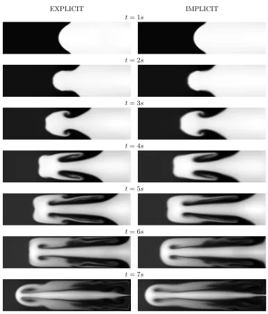
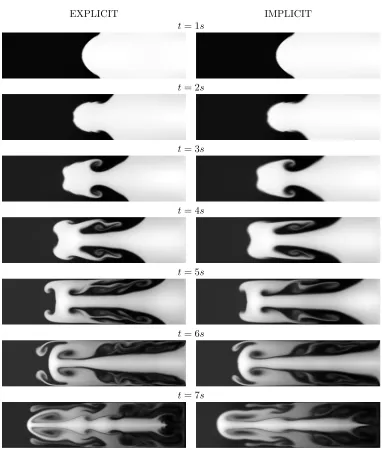
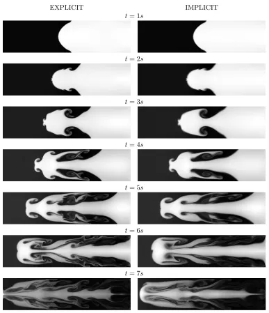
With such settings, the experiment runs as displayed on Figures 1 to 3. These figures show the evolution of the instability from t = 0s to t = 7s, as modeled by the explicit (on the left) and implicit (on the right) schemes, for different spatial refinements. We will come back to these figures after giving some remarks on the discretization used.
4.2.
Discretization
For the spatial discretization, we employ a uniform mesh with square cells (edge length ∆x= ∆y) indexed with the subscripts (i, j). For the time discretization, the time step length is re-evaluated at the end of each time iteration, proceeding as follows: first the CFL limit is computed classically according to
cfl limit = min
(i,j)
cs(i,j)+|ux|(i,j)
∆x +
cs(i,j)+ uy
(i,j)
∆y
−1
with the sound speed c2
s =γ(γ−1), |ux| and uy
the absolute value of the speed in thex- and y-directions,
respectively, and the minimum taken on all the mesh cells. Then, in the explicit case, the time step is taken as half the CFL limit:
dtexpl= 1
2cfl limit.
For the implicit case, the CFL limit can be overcome. In our study, the time step length is determined as a function of the relative variation ofρandE from one step to the next. More precisely, we define
dtimpl= min
δdtδrel
max
δdtmax(i,j) ∆ρ ρ
(i,j), δrel ,
δdtδrel
max
δdtmax(i,j) ∆E E
(i,j), δrel
cfl limit (8)
where, at time step n, ∆ρρ = ρnρn−1 −1, and similarly forE. To explain this formula, let us take two cases into
consideration:
• For small variations ofρandE, formula (8) reduces todtimpl=δdtcfl limit, so thatδdtdetermines the
time step length increase allowed in the implicit case. In the numerical tests reported here,δdtwas set
• For large variations ofρandE, formula (8) becomes
dtimpl= min
δrel
max(i,j) ∆ρ ρ (i,j)
,
δrel
max(i,j) ∆E E (i,j)
cfl limit (9)
so that δrel can be interpreted as the desired relative variations of the considered quantities (ρor E)
per time step: compared to the CFL limit, the time step will be reduced if the actual variations are larger thanδrel, and increased in the opposite case. In the numerical tests reported here,δrel was set
to 0.05.
4.3.
Qualitative results
We now look again at Figures 1 to 3, on each of which the same spatial mesh is used for both explicit and implicit schemes. We stopped the calculations after an evolution of 7sbecause, for now, we want to avoid (at least in the implicit scheme) the peculiarities appearing after the dense fluid has hit the left face (x= 0).
We first concentrate on the effect of mesh refinement for both schemes. Mesh refinement affects the shape of the curls appearing on the plots, this effect becoming more visible as the system evolves. Also, starting at around 4sof evolution, we notice the effect of mesh refinement on the distance achieved by the dense fluid in the lighter one at a given time of the evolution.
Then, we compare the explicit and implicit solutions for a given mesh refinement. The general evolution trend is satisfyingly similar, even though the implicit results appear more diffusive than the explicit ones. Also, discrepancies between the explicit and implicit solutions become prominent after 7sof evolution.
We conclude that comparing performance results between the explicit and implicit schemes is a difficult task in absolute terms: determining the appropriate mesh refinement for each scheme, as well as the appropriate time step length, should be done in view of the target result(s) of interest. Therefore, in the quantitative results below, we restrict our attention to the costs per finite volume cell and per time step for both schemes.
Finally, note that unphysical dissymmetries appear at evolution timest= 6sandt= 7sin the implicit case, when the 4096×1024 mesh is used. This might probably be due to round-off errors affecting the symmetry of the Jacobian system, and therefore not inherent to the implicit method itself.
4.4.
Quantitative Results
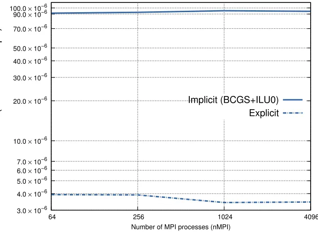
Figures 4 and 5 respectively present weak and strong scaling results obtained using 64 to 4096CPU cores, each core being assigned one MPI task.
We ran our calculation on the Jade supercomputer hosted by the French CINES computing center. The
CPUnodes used were 3 GHz Intel Xeon Quad-Core E5472 (“Harpertown”). In terms of running time, we were
limited to 24 hours. In order to obtain comparable results, the same evolution time was used for all runs: we limited our calculations to 2.844sof evolution, which corresponds to the evolution time reached after a 24 hour run onJade for the most time-consuming implicit run (16384×4096 mesh on 64 cores). Note that our explicit runs were typically longer than the implicit ones for the same grids, which means that all of the explicit runs did not reach the 2.844sevolution time. However, this does not affect our results in terms of cost per cell and per time step because, while in the implicit case this cost takes some evolution time before reaching a relatively constant value, it is not the case in the explicit case, where this cost appears constant from the start of the evolution. It appeared therefore more appropriate to use the full extent of our 24 hour runtime onJade in the implicit case.
4.4.1. Weak Scaling
Figure 4 displays the cost per cell and per time step, employing 64, 256, 1024 and 4096 cores, each of these cores dealing with a 128×128 square sub-domain. In turn, this corresponds to 4 different meshes for the whole domain, from 2048×512 to 16384×4096, all of them satisfying the 4-to-1 aspect ratio of the physical problem. We observe that weak scalability is well achieved by the explicit scheme, but not so well by the implicit one. This can be blamed on the loss of performance of the ILU(0) preconditioner: the average number of
BiCGStab inner iterations per time step increases from 8 with 64 cores to 19 with 4096 cores.
As expected, the cost per cell and per time step is higher using the implicit scheme rather than the explicit one: from 16 times on 64 cores to 27 times on 4096 cores. This extra cost per time step is clearly compensated in our tests by the longer implicit time step, but, as stated above, we prefer to avoid comparing implicit and explicit schemes in absolute terms, i.e., without a clear target result.
It is important to mention here that results on 4096 cores (and to a lesser extent those on 1024 cores) highly depend on the workload of the Jade supercomputer: results shown here are the best ones (i.e., were obtained on Sundays), and could be up to 2 to 3 times worse in terms of cost on heavy workload days. Results on 64 and 256 cores did not exhibit such dependency on the workload.
4.4.2. Strong Scaling
Figure 5 displays cost per cell and per time step for a 16384×4096 mesh, using 64 to 4096 cores. Strong scal-ability is well achieved by both explicit and implicit schemes. For the latter, the average number of BiCGStab inner iterations per time step remains nearly constant: from 17 with 64 cores to 19 with 4096 cores. Similarly the extra cost per cell and per time step for using the implicit scheme remains nearly constant (factor 23 to 27). Note that here again dependency on the workload was observed for large number of nodes, and only the best results are displayed.
5.
Conclusions and Perspectives
An implicit version of the explicit scheme of Vides et al. [8] was presented. A good qualitative agreement between the explicit and implicit solutions was observed, even if discrepancies between them, very limited at start, appeared to grow along the evolution. Using the implicit scheme rather than the explicit one implies an increase in cost per cell and per time step by a factor that turned out to range from 16 to 27 in our calculations, depending on the number of CPU cores employed. Nevertheless, this extra cost could be, at least in our tests, compensated by a longer time step. However, performance comparisons between both schemes should not be done in absolute terms, the appropriate space and time refinement for each scheme being highly dependent on the target result(s) of interest in production runs.
Our numerical results show that, while weak and strong scalabilities are both achieved by the explicit scheme, the proposed implicit scheme achieves strong but not weak scalability. This can be blamed on the lack of scalabil-ity of the localILU(0)preconditioner used to solve the Jacobian system. Therefore, other local preconditioners available inPETSc, as well as direct solvers interfaced by it, like MUMPS, SuperLU and PaStiX, should be considered. Moreover, global preconditionings other than block Jacobi need to be tested (e.g., Algebraic Schwartz Method with various overlaps) as well as Krylov accelerations other thanBiCGStab (e.g. GMRES). Using the full potential of thePETSclibrary will then hopefully provide full scalability. In turn we would have demonstrated the possibility to derive an implicit version of a given explicit scheme in a relatively easy way, given the ease of use of theTAPENADEtool used to derive the Jacobian matrix.
References
[1] Satish Balay, Jed Brown, Kris Buschelman, Victor Eijkhout, William D. Gropp, Dinesh Kaushik, Matthew G. Knepley, Lois Curfman McInnes, Barry F. Smith, and Hong Zhang. PETSc users manual. Technical Report ANL-95/11 - Revision 3.3, Argonne National Laboratory, 2012.
EXPLICIT IMPLICIT
t= 1s
t= 2s
t= 3s
t= 4s
t= 5s
t= 6s
t= 7s
Figure 1. Rayleigh-Taylor instability computed with the explicit and implicit schemes with a 1024×256 mesh. Computations performed on 16 processors.
[3] Satish Balay, William D. Gropp, Lois Curfman McInnes, and Barry F. Smith. Efficient management of parallelism in object oriented numerical software libraries. In E. Arge, A. M. Bruaset, and H. P. Langtangen, editors, Modern Software Tools in Scientific Computing, pages 163–202. Birkh¨auser Press, 1997.
[4] M. Gonz´alez, E. Audit, and P. Huynh. HERACLES: a three-dimensional radiation hydrodynamics code.Astronomy & Astro-physics, 464:429–435, 2007.
EXPLICIT IMPLICIT
t= 1s
t= 2s
t= 3s
t= 4s
t= 5s
t= 6s
t= 7s
Figure 2. Rayleigh-Taylor instability computed with the explicit and implicit schemes with a 2048×512 mesh. Computations performed on 64 processors.
[6] Inria Tropics team. TAPENADE Web page, 2012. http://www-tapenade.inria.fr:8080/tapenade/index.jsp and http://www-sop.inria.fr/tropics.
[7] N. Vaytet. HERACLES Web page.
http://irfu.cea.fr/Projets/Site heracles/index.html.
EXPLICIT IMPLICIT
t= 1s
t= 2s
t= 3s
t= 4s
t= 5s
t= 6s
t= 7s
2.0 × 10⁻⁶ 3.0 × 10⁻⁶ 4.0 × 10⁻⁶ 5.0 × 10⁻⁶ 6.0 × 10⁻⁶ 7.0 × 10⁻⁶ 10.0 × 10⁻⁶ 20.0 × 10⁻⁶ 30.0 × 10⁻⁶ 40.0 × 10⁻⁶ 50.0 × 10⁻⁶ 60.0 × 10⁻⁶ 70.0 × 10⁻⁶ 100.0 × 10⁻⁶
64 256 1024 4096
nMPI
×
Time / (nCells
×
nSteps)
Number of MPI processes (nMPI)
Implicit (BCGS+ILU0) Explicit
Figure 4. Weak scaling for the Rayleigh-Taylor instability: each core deals with a 128×128 square sub-domain. Therefore meshes range from 2048×512 (for nMPI=64) to 16384×4096 (for nMPI=4096).
3.0 × 10⁻⁶ 4.0 × 10⁻⁶ 5.0 × 10⁻⁶ 6.0 × 10⁻⁶ 7.0 × 10⁻⁶ 10.0 × 10⁻⁶ 20.0 × 10⁻⁶ 30.0 × 10⁻⁶ 40.0 × 10⁻⁶ 50.0 × 10⁻⁶ 70.0 × 10⁻⁶ 90.0 × 10⁻⁶ 100.0 × 10⁻⁶
64 256 1024 4096
nMPI
×
Time / (nCells
×
nSteps)
Number of MPI processes (nMPI)
Implicit (BCGS+ILU0) Explicit