Determination of Spatial-Temporal Correlation
Structure of Troposphere Ozone
Data in Tehran City
S.S. Mousavi and M. Mohammadzadeh
*Departmentof Statistics, Faculty of Science, Tarbiat Modares University, Tehran, Islamic Republic of Iran
Received: 20 March 2013 / Revised: 6 April 2013 / Accepted: 14 May 2013
Abstract
Spatial-temporal modeling of air pollutants, ground-level ozone concentrations
in particular, has attracted recent attention because by using spatial-temporal
modeling, can analyze, interpolate or predict ozone levels at any location. In this
paper we consider daily averages of troposphere ozone over Tehran city. For
eliminating the trend of data, a dynamic linear model is used, then some features
of correlation structure of de-trended data, such as stationarity, symmetry and
separability are considered. Next based on the obtained features, an appropriate
model is proposed. This model can be used for future predictions of ozone in
Tehran.
Keywords: Spatial-temporal process; Dynamic spatial linear model; Stationary; Symmetry; Separability
* Corresponding author, Tel.: +98(21)82883483, Fax: +98(21)82883483, E-mail: [email protected]
Introduction
In recent years there has been a tremendous growth in the statistical models and techniques to analyze environmental processes that are spatially and temporally indexed, such as air pollution data. Troposphere Ozone is a secondary pollutant that results from photochemical reactions involving nitrogen oxides (NOx) and volatile organic compounds (VOC’s). The rate of ozone production depends on meteorological conditions, primarily sunlight, temperature, along with wind speed and direction. Therefore its levels are difficult to control. A complete description of the chemical processes involving ozone can be found in Seinfeld and Pandis [24]. In 1997, the U.S. Environmental Protection Agency (U.S. EPA) defined the National Ambient Air Quality Standards (NAAQS)
for ozone in terms of the daily 8-hour maximum ozone measurement among the network of monitoring sites covering a given area. The new standard is defined in terms of the 3-year rolling average is less than 80 parts per billion (ppb), (see e.g. epa.gov/air/criteria. html).
considerably simplify fitting a covariance model to the data. But often they are not applicable, for example with ozone data, separability is not generally a realistic assumption. Nonseparable spatial-temporal covariance models have been proposed by Christakos and Hristopulos [3], Cressie and Huang [7], Christakos [2], De Cesare et al. [8,9], Ma [16, 17, 18, 19], Gneiting [11] and Stein [25].
Cressie and Huang [7] based their approach on Fourier transforms. Gneiting [11] proposed another general class of nonseparable, stationary covariance functions for spatial-temporal random processes directly in the spatial-temporal domain. In both these papers the spatial-temporal processes are assumed stationary in time and spatial components. Since the trend of the data arises bias on the covariance function estimation (Cressie [6]), it is necessary to use the de-trended data for fitting a valid covariance function. In this paper, we use a dynamic spatial linear model for modeling trend of ozone data in Tehran city, one of the most polluted cities in Iran. Next, according to the obtained features for correlation structure of this data, a suitable function for covariance structure of the de-trended data is fitted.
In this paper, first, introduce some basic features of the spatial-temporal theory. Next, pertinent exploratory analyses of the data is presented. Our proposed model for modeling trend of spatial-temporal data is described in the Spatial-Temporal Trend section. Then the features of correlation structure of the ozone concentration in Tehran city are specified and a suitable spatial-temporal covariance function is fitted. Finally, Results and Discussion are given.
Background: Spatial-Temporal Process
Let Z
,
Z
s, ;t sR td, R
denotes aspatial-temporal random field, where s represents a site in d-dimensional space and t represents time. In general, a spatial-temporal random field can be decomposed as
1 ,1
, 2 , 2
dt t R R
s s
Definition 2. The zero mean spatial-temporal process
,t s has stationary covariance if
1, ; , 2 1 2
;C s s t t C h u ;
h ; u Rd Rwhere h s 1 s2 and u t1 t2.
Definition 3. The spatial-temporal process
s,t has aseparable covariance if there exist purely spatial and purely temporal covariance functions CS and CT ,
respectively, such that
1, ; t , t2 1 2
CS
1 , 2
C t , tT 1 2
C s s s s ;
1 ,1
, 2 , 2
dt t R R
s s
Definition 4. The spatial-temporal process
s t, hasfully symmetric covariance if
1 , ,1
2 , 2
1 , 2
, 2 , 1
Cov s t s t Cov s t s t
for all spatial-temporal coordinates
s t1 ,1
and
s t2 , 2
ind
R R (Gneiting [11]; Stein [25]). Also, a
stationary spatial-temporal covariance function is fully symmetric if
C
h , u = C(h ,−u) = C (−h, u) = C (−h,−u);
h , u RdRExploratory Analysis
Figure 1. Monitoring sites in Tehran city. Figure 2. Box plot of the data at 9 sites.
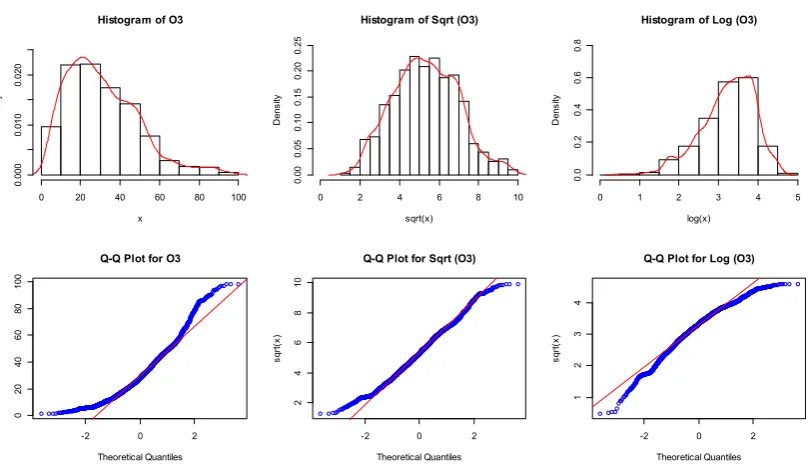
Figure 3. Histograms and Normal QQ plots for original, square root and logarithmic data.
Tehran city. Fig. 1, shows the geographical locations of these 9 stations over map of Tehran city. Between initial hourly data, some points were missing observation which we imputed them by using of average method, that is, missing observations at each station, is imputed by daily average of all data at the same station.
The box-plot of the data in each station, plotted in Fig. 2, shows considerable spatial variations in this data set. It also shows that the sites 1 and 5 are more and less polluted than others, respectively. Because site 1 is in central area and messy of this city and site 5 is in suburbia out of the city.
For analysis of spatial-temporal data, it is necessary
to consider their normality, stationarity and homo-geneity of the variance. Empirical analysis suggested that normality was a reasonable assumption for air pollutant data. For considering normality, the histogram, normal QQ plot and Shapiro-Wilk test for original, square root and logarithm of the data are used. Both of this plots and result of the Shapiro-Wilk test showed that the original and logarithmic data have asymmetric distribution and transformed data by the square root transformation has nearly symmetric distribution (Fig. 3). Also the p-value of Shapiro-Wilk test for the square root of the data is more than 0.05 that approve normality of the transformed data. Therefore we use normal
Histogram of O3
x
D
ens
ity
0 20 40 60 80 100
0.
00
0
0.
01
0
0.
02
0
Histogram of Sqrt (O3)
sqrt(x)
D
ens
ity
0 2 4 6 8 10
0.
00
0.
05
0.
10
0.
15
0.
20
0.
25
Histogram of Log (O3)
log(x)
D
ens
ity
0 1 2 3 4 5
0.
0
0.
2
0.
4
0.
6
0.
8
-2 0 2
0
20
40
60
80
100
Q-Q Plot for O3
Theoretical Quantiles
x
-2 0 2
24
68
10
Q-Q Plot for Sqrt (O3)
Theoretical Quantiles
sq
rt
(x
)
-2 0 2
1
234
Q-Q Plot for Log (O3)
Theoretical Quantiles
sq
rt
(x
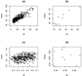
al. [12] used the plot of standard deviations versus the mean of data (over time) for considering homogeneity of variance. By plotting the standard deviation against the mean of the original data over the 365 time instants analyzed, in Fig. 5.a and over 9 sites in Fig. 5.b, perceive that variance increases as mean increases. Therefore variance of the original data is not homogen. But for the square root of data there is no specific pattern in Fig. 5.c and Fig. 5.d, so the variance of the transformed data is homogen.
Spatial-Temporal Trend
For inquiring symmetry and separability of spatial-temporal covariance function, it is needful that eliminate the trend of data. There are variety methods for trend modeling. Cox and Chu [5] used a generalized linear model approach to estimate trends in daily maximum ozone levels. Stroud et al. [23] modeled the trend at each time-period as a locally weighted mixture of linear regressions. Huerta et al. [14] and Zheng et al. [29] applied a dynamic linear model to explain ozone trends. Fuentes et al. [10] introduced spectral spatial-temporal models, using covariates that have spatial-temporal dynamic coefficients and applied ambient ozone data provided by U.S. EPA in their article.
Comparing four different models for trend of the ozone data during 2009, Mousavi And Mohammad-zadeh [20] proposed a dynamic spatial linear model. In this section, we used the same spatial-temporal model for the transformed data. Then after de-trending the data, in the next section, the symmetry and separability of spatial-temporal structure of the data are considered.
Dynamic Spatial Linear Model
Let the m-dimensional observation vector Z
t
Z s1, , ,t Z sm,t
at time point t , 1, ,t n,has multivariate Normal distribution Nm
μ
t ,Vt
.with m m covariance matrix V t ,Gt is the evolution
matrix related to the state vector and ω
t is the evolution error vector with q q covariance matrix Wt,also
t and ω
t are independent. This model isFigure 5. Variation of standard deviation against the mean of the original data (a,c), and square root of data (b,d).
completed with a prior on the initial state vector,
0| 0 ~ 0, 0 ,
θ D N m C where D0 denotes the initial
information set, and m0 and C0 are known (West and
Harrison [27]). Assume that the spatial-temporal observations have cyclical behavior and the state vector can be define as
1
, 2
' '
θ t θ t θ t ' , where q = r +
2k, '
1 t is the r1 spatial process and 2k1 -dimensional vector '
2 t
describe cyclical of data. Coefficients of the spatial process characterized with X
that inclusive length, width, height and other covariates. Corresponding to this partitioning for
t , consider design matrix as '
, 1, ,
k
t t t t
F X F F , where each of the Fth , h1, , k , are m2 matrix that all of elements of the first column are 1 and second column are 0. Therefore for evolution matrix Gt can be used a
block structure with blockdiag
, 1, ,
k
t r r t t
G I G G ,
where each of the blocks Gth , h1, , k , is a 2 2
harmonic matrix of the form
2 / 2 /
, 1, ,
2 / 2 /
h
t
cos h p sin h p
G h k
sin h p cos h p
For modeling the spatial dependency of the observations, consider the covariance matrix 2
t
V V, where V exp V
/
and elements of V is determined by a known spatial correlation function, as Matern correlation function. The evolution variance Wtcan be specified either explicitly or through a discount factor
0,
, which defines Wt Pt , where
1( 1 | )
t t t
P var G t D . A discount factor of 0
gives a static model, with the same coefficients for all time periods, whereas implies coefficients which are independent over time, i.e. no temporal smoothing at all (Stroud et al. [23]).
Trend of Ozone Data
Let Z
si,tj
denotes the square root of observedozone data, at each spatial location si , i 1, ,9 and each time tj T
1, ,365
. For modeling the trend of the data, we use the available important meteorological variables in monitoring stations, i.e. NOmember of θ
t is simulated from autoregressive model given by
1
, 1, 2,3.i t i t i t i
The observation errors are assumed to be Gaussian, with mean 0 and covariance 2
t
V V I , where I is identity matrix of order 9. Leaving 2 unknown, we
select a Gamma prior: 12 ~ Gamma
0.01 , 0.01
so that
its mean is 1 and its variance is large. Since usual selection prior for is the Uniform distribution
,U a b , where a and b are minimum and maximum
values of spatial lag, we used ~ U
0.051,0.315
where 0.051 and 0.315 are Transformed numbers by Lambert transformation. To complete the model specification, we choose a diffuse prior for the initial state vector: 0 |
D0 ~ N3
0,100I
, where I is a 3 3identity matrix. Next the MCMC algorithm was run for 10000 iterations. After a burn in period of 5000 iterations, the Bayesian estimation of the parameters were obtained as shown in Table 1 and also R2 0.94.
Correlation Structure of Ozone Data
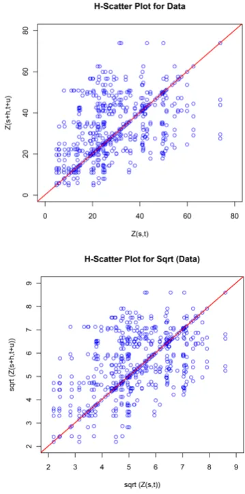
To investigate the spatial-temporal correlation structure of the data, first we used a nonparametric test where proposed by Shao and Li [21] to test for symmetry and separability of spatial-temporal covariance functions (Behshad and Mohammadzadeh [1]). Using this testing for the de-trended data, rejected the assumption of separability and didn’t reject the assumption of fully symmetry at 5% level. Also H-scatter plot for the de-trended data appear where there is stationary in spatial-temporal covariance structure of this de-trended data. Therefore we consider a symmetric, nonseparable and stationary spatial-temporal covariance function for the ozone data.
2 2 2 2 2 2 , exp 1 1 d b C u au au h h
2
2 2 2 2
3 , exp
C h u au b h cu h
where a 0 and b 0 are the scale parameters of the time and spatial lags, respectively, c 0, and
2 C 0,0
. Their approach is novel and powerful but depends on Fourier transform pairs in Rd. In other
words, it is restricted to a comparably small class of functions for which a closed-form solution to the d -variate Fourier integral is known.
The approach of Cressie and Huang [7] was taken by Gneiting [11], but the aforementioned limitation is avoided and very general classes of valid spatial-temporal covariance models are provided. He applied completely monotone functions and positive functions with a completely monotone derivative. Using his method four covariance functions in RdR were
considered as follows
2 2 4 2 2 2 , exp 1 1 d b C u a u a u h h
5 ,C h u
2 2 2 2 2 2 2 1 1 exp db c a u
c a u
a u c a u c
7 ,
C hu
2 2 2 2 2 2 2 1 1 1 db c a u
c a u
a u c a u c
h
where a and b are nonnegative scale parameters of time and spatial lags, respectively and 0 c 1. The smoothness parameters and take values in (0,1],
β is spatial-temporal interaction parameter where take values in [0,1], 2 is the variance of the
spatial-temporal process and 0. Kent et al. [15] draw our attention on the counterintuitive presence of a dimple in the spatial-temporal covariance surface in certain cases. That is for a fix spatial lag the temporal covariance is not a decreasing function of the temporal lag as one would normally expect. So we should be careful in applications that the dimple does not accrue at relevant lags.
A weighted-least-squares (WLS) method (Cressie [6]) is used to estimate parameters of each of seven covariance models‚ by minimizing the criterion given by
1 2 2 , , 2, ' 1 ,
, ( , | )
( , | ˆ
)
U
i i i i
i i u i i
C u C u
W C u
h h θθ
h θ
over all possible θ. Here hi i, is the spatial lag
between stations i and i’, and u is the temporal lag.
, ,
ˆ
i i
C h u is the empirical correlation given by
ˆ , 1
, C u N u h h , , , ,
, ,i j i j
i j i j N u
Z t Z Z t Z
h s s where
' , , , , : ;; , 1, , ; , 1, ,
i i
j j
N u i i j j Tol
t t u i i m j j n
h s s h
Here Tol
h
is some specified tolerance region around h
, and N h
,u
is the number of distinct elements in N
h
, ;u
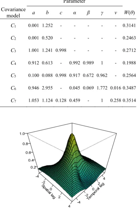
1, , , 1, ,L u U .Table 2 displays comparable parameter estimates for the seven models. Based on the smallest WLS value of
W θ , model 4 provides the closest fit to spatial-temporal covariance of ozone data in Tehran city, which its three 3D plot is shown in Fig. 6.
Results and Discussion
Since ozone concentration data depend to spatial and time locations of observations, we have used a dynamic linear model for modeling trend of these data. After de-trending the data, using the test of Shao and Li [22] shows symmetry and nonseparability of spatial-
Table 1. Estimation of the model parameters
Parameter θ1(0) θ2(0) θ3(0) σ λ
Estimated -0.0295 1.3067 0.1083 0.1584 0.1834
Table 2. Estimates of the Parameters of Different Covariance Functions
Parameter Covariance
model a b c α β γ ν W(θ)
C1 0.001 1.252 - - - 0.3141
C2 0.001 0.520 - - - 0.2463
C3 1.001 1.241 0.998 - - - - 0.2712
C4 0.912 0.613 - 0.992 0.989 1 - 0.1988
C5 0.100 0.088 0.998 0.917 0.672 0.962 - 0.2564
C6 0.946 2.955 - 0.045 0.069 1.772 0.016 0.3487
C7 1.053 1.124 0.128 0.459 - 1 0.258 0.3514
Figure 6. Surface of spatial-temporal covariance of Model 4.
Sp atial la
g -4 -2 0 2 4 Tem pora
l lag
Acknowledgement
The authors are thankful to the referees for their valuable comments that improved this paper. Partial support from Ordered and Spatial Data Center of Excellence of Ferdowsi University of Mashhad is also acknowledged.
References
1.Behshad, E. and Mohammadzadeh, M. Evaluation of Tests for Separability and Symmetry of Spatio-Temporal Covariance Function, Journal of Statistical Research of Iran, 8: 1-27 (2011).
2.Christakos, G. Modern Spatiotemporal Geostatistics, Oxford University Press, Oxford, 288 p (2000).
3.Christakos, G. and Hristopulos, D. T. Spatio-Temporal Environment Health Modeling: A Tractatus Stochasticus: Kluwer, Boston, 424 p (1998).
4.Cocchi, D., Fabrizi, E. and Trivisano, C. A Stratified Model for the Assessment of Meteorologically Adjusted Trends of Surface Ozone, Environmental and Ecological Statistics, 12: 1195–1208 (2005).
5.Cox, W. M. and Chu, S. H. Meteorologically Adjusted Ozone Trends in Urban Areas: A Probabilistic Approach,
Atmospheric Environment, 27: 425– 434 (1992).
6.Cressie, N. Statistics for Spatial Data, Wiley, New York (1993).
7.Cressie, N. and Huang, H. C. Classes of Nonseparable, Spatio-Temporal Stationary Covariance Functions:
Journal of the American Statistical Association, 94: 1330– 1340 (1999).
8.De Cesare, L., Myers, D. E. and Posa, D. Estimating and Modeling Space–Time Correlation Structures: Statistics and Probability Letters, 51: 9–14 (2001a).
9.De Cesare, L., Myers, D. E. and Posa, D. Product-Sum Covariance for Space–Time Modeling: An Environmental Application: Environmetrics, 12: 11–23 (2001b).
10.Fuentes, M., Chen, L. and Davis, J. M. A Class Non-separable and Nonstationary Spatial-Temporal Covariance Function, Environmetrics, 19: 487– 507 (2008).
11.Gneiting, T. Nonseparable, Stationary Covariance Functions for Space-Time Data. Journal of the American Statistical Association, 97: 590 – 600 (2002).
12.Huang, H. C., Martinez, F., Mateu, J. and Montes, F. Model Comparison and Selection for Stationary
Space-Covariance Models, Journal of Statistical Planning and Inference, 116: 489 – 501 (2002.b).
18.Ma, C. Nonstationary Covariance Functions that Model Space–Time Interactions, Statistics and Probability Letters, 61: 411– 419 (2002.c).
19.Ma, C. Recent Developments on the Construction of Spatio-temporal Covariance Models, Stochastic Envionmental Research, Vol. 22, Supplement 1, 39–47 (2008).
20.Mousavi, S. S. and Mohammadzadeh, M. Spatial-Temporal Trend Modeling for Ozone Concentration in Tehran City, Journal of Statistical Research of Iran, Vol.
8: No 2, 177–191 (2011).
21.Sahu, S. K., Gelfand, A. E., and Holland, D. M. High Resolution Space-Time Ozone Modeling for Assessing Trends, Journal of American Statistical Society, 102: 1221–1234 (2007).
22.Shao, X., and Li, B. A Tuning Parameter Free Test for Properties of Space-Time Covariance Function, Journal of Statistical Planning and Inference, 139: 4031– 4038 (2009).
23.Stroud, R. J., Muller, P., and Sanso, B. Dynamic Models Spatio-Temporal Data, Journal of the Royal Statistical Society, Series B, 63: 673– 689 (2001).
24.Seinfeld, J. H. and Pandis, S. N. Atmospheric Chemistry and Physics: from Air Pollution to Climate Change, Wiley- Inter science: New Jersey (1998).
25.Stein, M. L. Space-Time Covariance Functions, Journal of American Statistical Association, 100: 310–321 (2005). 26.Thompson, M. L., Reynolds, J., Cox, L. H., Guttory, P.
and Sampson, P. D. a Review of Statistical Methods for the Meteorological Adjustment of Tropospheric Ozone.
Atmospheric Environment, 35: 617– 630 (2001).
27.West, M., and Harrison, J. Bayesian Forecasting and Dynamic Models, Springer-Verlag, New York (1997). 28.Wikle, C. K. Hierarchical Models in Environmental
Science. International Statistical Review, 71: 181–1990 (2003).
29.Zehang, J., Cox, W. M and Davis, J. M. Internal Variation in Meteorological Adjusted Ozone Levels in the Eastern United State, Atmospheric Environment, 41: 705-716 (2007).