Analytical discrete optimization

© Shiraz University

ANALYTICAL DISCRETE OPTIMIZATION

*

M. HATAM AND M. A. MASNADI-SHIRAZI

* * Dept of Electrical Engineering, Shiraz University, Shiraz, I. R. of Iran

Email: [email protected] Email: [email protected]

Abstract– Although for many years scientists and engineers have been faced with the problem of optimizing discrete functions, no general analytical method has been proposed for multidimensional discrete optimization. All the methods that have already been reported in the literature are algorithmic. In one dimensional discrete optimization, no general analytical method has yet been proposed to find all the local minima and maxima of multimodal one dimensional discrete functions either. In this paper, for the first time, a general analytical method has been proposed for solving multidimensional and multimodal discrete optimization problems. Here, first we will introduce the method and present its mathematical proof, and then confirm its validity through some examples and computer simulations.

Keywords–Discrete optimization, multimodal optimization

1. INTRODUCTION

Nowadays, optimization is one of the most interesting branches of science that is useful in many applied problems in engineering, mathematics, computer science, physics, and so on. One of the most important branches of optimization is discrete optimization (or integer optimization) which deals with the methods of optimizing functions with integer variables. No general method has yet been proposed to analytically evaluate the minima and maxima of multidimensional discrete functions. All the known methods have been developed based on algorithmic approaches such as integer programming (IP) and searching, which are very complex and need a high order of computations [1-12]. In [13] an analytical method has been proposed for maximizing unimodal one dimensional discrete functions, however the author emphasized that the extension of his method to a multidimensional case would not be valid. In this paper we will introduce an analytical approach that is preferable to the known existing ones. Using this method, the local minima and maxima of the discrete functions would be evaluated by a single analytical formula, even if the function has infinite maxima and minima. This leads to an enormous reduction of the computational load, particularly in multidimensional cases, without using any suboptimal approach. The other advantage of using this analytical approach is in solving classic discrete optimization problems very easily without using any induction approach. If the discrete function has infinite minima and maxima distributed in an unconstrained domain, this approach is able to catch them analytically, where it is not possible to do so by using the IP and searching approaches because an unconstrained domain contains an infinite number of points.

In this paper, first we will introduce the methodology and present its mathematical proof, and then confirm its validity through some examples and computer simulations.

2. ANALYTICAL APPROACH

a) One dimensional discrete optimization

Definition of local minimum and maximum for discrete functions:

We say is a local minimum for the discrete function if , and are in the domain of

and we have:

*

n f[n] _n* _n*_{−1 n}*₊₁

] [n f

] 1 [ ]

[_n* _{≤ f n}*₋

f and _f[_n*]_{≤ f}[_n*₊1].

We say is a local maximum for the discrete function if , and are in the domain of

and we have:

*

n f[n] _n* _n*_{−1 n}*₊₁

] [n f

] 1 [ ]

[_n* _{≥ f n}*₋

f and _f[_n*]_{≥ f}[_n*₊1].

Theorem 1:

Suppose that f[n] is a discrete function defined on D⊂Z and is a continuous real function

defined on so that , and at each integer point such as

) (x fr

R

D

_r

⊂

D

⊂

D

_r

n

′

we have

f n

_r

( )

′

=

f n

[ ]

′

.

Let x1,x2,...,xm be all the solutions of the equation fr(x)− fr(x−1)=0. The set A consisting of the integer

parts of all ’s x_i (i=1, 2, … ,m ) plus all (x_i−1)’s when is integer contains all the local minima and

maxima of .

i x ]

[n f Proof:

Assume that is a local minimum of_n* _f[n]. We have:

* * * *

r r

* *

r r

f[n ] f[n

1]

f (n ) f (n

1)

f (n ) f (n

1) 0

≤

− ⇒

≤

−

⇒

−

− ≤

(1.1)

* * * *

r r

* *

r r

f[n ] f[n

1]

f (n ) f (n

1)

f (n

1) f (n ) 0

≤

+ ⇒

≤

+

⇒

+ −

≥

(1.2)

Since fr(x) is a continuous function, fr(x−1) is also a continuous function and therefore

is a continuous function. According to (1.1) and (1.2) we have and

. Since is a continuous function it has at least one root in the interval . Thus,

the equation has at least one solution in the interval . If the solution(s) is

(are) in the interval then the integer part of the solution(s) would be , and if the solution is

equal to then and would be in the set A. Thus, in each case the set A contains

the local minimum .

) 1 ( ) ( )

(x =Δ f x − f x−

g _{r r g}(_n*)_≤0

0 ) 1 (_n*_{+ ≥}

g g(x) [_n*,_n*₊1]

0 ) 1 ( )

(x − f x− =

f_{r r} [_n*,_n*₊1]

) 1 ,

[_n* _n*_{+ n}*

1 *₊

n _n*₊1 _(n*_+1)−1=n* *

n

Assume that is a local maximum of _n* _f[n]. We have:

* * * *

r r

* *

r r

f[n ] f[n

1]

f (n ) f (n

1)

f (n ) f (n

1) 0

≥

− ⇒

≥

−

⇒

−

− ≥

(2.1)

* * * *

r r

* *

r r

f[n ] f[n

1]

f (n ) f (n

1)

f (n

1) f (n ) 0

≥

+ ⇒

≥

+

⇒

+ −

≤

(2.2)

According to (2.1) and (2.2) we have and , thus the continuous function

has at least one root in the interval . Therefore, the equation

has at least one solution in the interval . If the solution(s) is (are) in the

interval then the integer part of the solution(s) would be and if the solution is equal to

0 ) (_n* _≥

g _g(_n*₊1)_≤0 )

1 ( ) ( )

(x =Δ f x − f x−

g r r [ , 1]

* * _{n +} n 0

) 1 ( )

(x − f x− =

fr r [ , 1]

* * _{n +} n )

1 ,

[_n* _n*_{+ n}* _n*_+1,

then and would be in the set A. Therefore in each case the set A contains the local

maximum .

* ₁

n + _(n*_{+ − =1) 1 n}*

* n

Note: In theorem 1, in the case that some of the solutions of fr(x)− fr(x−1)=0, as , are integer we

have:

i x

( ) ( 1) 0

[ ] [ 1] 0

[ ] [ 1]

r i r i i i

i i

f x f x f x f x f x f x

− − =

⇒ − − =

⇒ = −

Thus, if is a maximum (minimum) of xi f[n], then

x

i

−

1

is equivalently another maximum (minimum) of

with the same value.

] [n f

Note: Suppose has global minimum or maximum. If the set A in theorem 1 consists of only one

number as , then is the global minimum or global maximum of . If the set A consists of only

two successive numbers as and , for which

] [n f * 1

n *

1

n f[n]

* 1 1

n − *

1

n f n[ ]₁* = f n[ ₁*−1], then *

1 1

n − and are the global

minima or global maxima of .

* 1 n ]

[n f

Note: When the discrete function is given by a mathematical formula we can use the same formula

for by substituting discrete variable with real variable

] [n f )

(x

fr

n

x

whenever the resulting

f x

r

( )

is a

continuous function. In this case we name

f x

_r

( )

as f x( ). For example, if _{f n[ ]=n}2 _{we can choose}

2

( ) ( )

r

f x = f x =x . We use the notation:

( [ ])

( )

(

1)

r

r r

f

dif f n

=

f x

−

f x

−

But when f xr( ) has the same formula as f n[ ], we drop the index in the above notation and use the

notation:

r f

( [ ])

( )

(

1)

dif f n

=

f x

−

f x

−

1. Properties of the operator dif: When f xr( )= f x( ) has the same formula as f n[ ], we can state the

following properties for the operator dif.

1- dif (C) = 0 when C is a constant

Proof:

[ ] , ( )

( ) 0

f n C f x C

dif C C C

= =

⇒ = − =

2- dif (an) = a when a is a constant

Proof:

[ ] , ( )

( ) ( 1)

f n an f x ax dif an ax a x a

= =

⇒ = − − =

3- Linearity:

1 1 2 2 1 1 2 2

1 2

(

[ ]

[ ])

( [ ])

( [ ])

where ,

and

areconstants

dif a f n

a f n

a dif f n

a dif f n

a

a

+

=

+

Proof:

1 1 2 2

1 1 2 2

1 1 2 2 1 1 2 2

1 1 1 2 2 2

1 1 2 2

[ ]

[ ]

[ ]

( )

( )

( )

( [ ])

( )

( ) (

(

1)

(

1))

( ( )

(

1))

( ( )

(

1))

( [ ])

( [ ])

f n

a f n

a f n

f x

a f x

a f x

dif f n

a f x

a f x

a f x

a f x

a f x

f x

a f x

f x

a dif f n

a dif f n

=

+

=

+

⇒

=

+

−

− +

=

−

−

+

−

−

=

+

Example 1:

Find the maximum(s) of the function _⎟⎟, where the domain of is

⎠ ⎞ ⎜⎜ ⎝ ⎛ = n k n

f[ ] f {n|n∈Z, 0≤n≤k}. Since n!=Γ(n+1) we have:

) 1 ( ) 1 ( ) 1 ( )! ( ! ! ] [ n k n k n k n k n k n f − + Γ + Γ + Γ = − = ⎟⎟ ⎠ ⎞ ⎜⎜ ⎝ ⎛ = The function ) 1 ( ) 1 ( ) 1 ( ) ( x k x k x f_r − + Γ + Γ + Γ

= is a continuous real function for 0≤x≤k because is a

continuous function for and we have

) (x

Γ

0

x> Γ(x+1)≠0 and Γ(k+1−x)≠0 for 0≤x≤k. At integer points

such as x n= ′ we have

f n

_r

( )

′ =

f n

[ ]

′

. Using theorem 1 to find the maximum(s) of f[n] we have:

) 1 ( ) 1 ( ) 1 1 ( ) ( 0 ) 1 1 ( ) ( ) 1 ( ) 1 ( )} 1 ( ) 1 ( ) 1 1 ( ) ( ){ 1 ( 0 ) 1 1 ( ) ( ) 1 ( ) 1 ( ) 1 ( ) 1 ( 0 ) 1 ( ) ( x k x x k x x k x x k x x k x x k x k x k x k x k x k x f x fr r

− + Γ + Γ = + − + Γ Γ ⇒ = + − + Γ Γ − + Γ + Γ − + Γ + Γ − + − + Γ Γ + Γ ⇒ = + − + Γ Γ + Γ − − + Γ + Γ + Γ ⇒ = − −

Using the property Γ(x+1)=xΓ(x)we can rewrite the above relation in the form:

) 1 ( ) ( ) 1 ( ) 1 )(

(x k+ −xΓ k+ −x =xΓ xΓ k+ −x

Γ

SinceΓ(x+1)≠0 and Γ(k+1−x)≠0 for 0≤x≤k we can divide both sides by these terms and obtain:

2 1 ) 1 ( + = ⇒ = − + k x x x k

According to theorem 1 the maximum(s) of the discrete function f[n] can be found by:

*

1 1

[ ] if is not integer

2 2

1 1 1

and 1 if is integer

2 2 2

k k

n

k k k

+ + ⎧ ⎪⎪ = ⎨ _{+ + +} ⎪ ₋ ⎪⎩

Where [.] denotes the integer part function and denotes the maximum(s) of _n* _f[n].

2 1

+

k _{is integer if and only if k is an odd number, thus:}

*

1 1

[ ] [ ] for k eve

2 2 2

1 1

and for k odd

2 2 k k n k k + ⎧ _{= +} ⎪⎪ = ⎨ _{+ −} ⎪ ⎪⎩ n

In the case of being even, k

2 k

is integer, hence:

*

for k even 2

1 1

and for k odd

k n

f[ ]=_⎜⎜⎛ _⎟⎟⎞ (1− ) − Example 2:

Find the maximum(s) of the Bernoulli distribution function

n_⎠

⎝ , where is a positive

integer constant and the domain of is

n k

n _p

p k

f {n|n∈Ζ, 0≤n≤k} and is a real constant and p 0< <p 1. Since n!=Γ(n+1) we have:

n k n

n k n

p p n k n

k

p p n k n

k n

f

− −

− −

+ Γ + Γ

+ Γ =

− −

=

) 1 ( ) 1 ( ) 1 (

) 1 (

) 1 ( )! ( !

! ] [

Similar to example 1, we can realize that the function x k x

r _{x k x} p p

k x

f − −

− + Γ + Γ

+ Γ

= (1 )

) 1 ( ) 1 (

) 1 ( )

( is a

continuous real function for 0≤x≤k. At integer points such as x=n' we have

f n

_r

( )

′ =

f n

[ ]

′

. Using

theorem 1 to find maximum(s) of f[n] we have:

1 1

1

( ) ( 1) 0

( 1) _{(1 )}

( 1) ( 1 )

( 1) _{(1 ) 0}

( ) ( 1 1)

( 1) (1 ) { ( ) ( 1 1

( 1) ( 1 ) (1 )} 0

r r

x k x

x k x

x k x

f x f x

k _{p p}

x k x

k _{p p}

x k x

k p p x k x

x k x p p

− − − + −

−

− − =

Γ +

⇒ −

Γ + Γ + − Γ +

− −

Γ Γ + − +

⇒ Γ + − Γ Γ + − +

−Γ + Γ + − − =

)

=

ince Γ(k 1) (1_{+ p}x _{− p})k x− _≠0 we have: S

1

( ) (x k 1 x 1) (x 1) (k 1 x p) − (1 p)

Γ Γ + − + = Γ + Γ + − −

Using the property Γ(x+1)=xΓ(x)we can rewrite the above relation in the following form:

1

( ){( 1 ) ( 1 )}

{ ( )} ( 1 ) (1 )

x k x k x

x x k x p− p

Γ + − Γ + −

= Γ Γ + − −

SinceΓ( ) 0x ≠ and Γ(k+1−x)≠0 for 0≤x≤k we can divide both sides by these terms and obtain:

1

1

1

( 1 ) (1 )

{ (1 ) 1} 1

( ) 1 ( 1

k x xp p

x p p k

x p k x p k

− −

−

+ − = −

⇒ − + = +

⇒ = + ⇒ = + )

According to theorem 1 the maximum(s) of the discrete function f[n] can be obtained as:

* [ ( 1)] if ( 1) is not integer

( 1) ( 1) 1 if ( 1) is integer

p k p k

n

p k and p k p k

+ +

⎧

= ⎨ _{+ + − +}

⎩

Where [.] denotes the integer part function and denotes the maximum(s) of _n* _f[n].

Example 3:

Find local maxima and minima of the functionf[n]=sin(n/3).

The function fr(x)=sin(x/3) is a continuous real function and at integer points such as x=n' we have

( ') [ ']

r

f n = f n . Using theorem 1 to find local maxima and minima of f[n] we have:

( [ ]) ( ) ( 1) 0 sin( / 3) sin(( 1) / 3)

1/ 2 3( 1/ 2) ,

r r dif f n f x f x

x x

x k π k

= − − =

⇒ = −

According to theorem 1, the local maxima and minima of the discrete function f[n] can be obtained from:

_n*_{=[1/ 2 3(+ k−1/ 2) ]π ,k∈ Ζ}

Where [.] denotes the integer part function and shows the local maxima and minima of . Note that

the term 1/

*

n f[n]

2 3(+ k−1/ 2)π is always non-integer because π is irrational and the result of adding or multiplying an irrational number by a nonzero rational number is irrational, and hence, non-integer.

0 5 10 15 20 25 30 35 40 45 50

-1 -0.5 0 0.5 1

n

si

n(n

/3)

Fig. 1. Plot of sin(n/3) versus n. The filled points represent maxima and minima of sin(n/3) for k=1,2,…,5

2. Necessary and Sufficient condition for local minima and maxima: In few cases, the set A obtained

from theorem 1 may contain some additional points rather than maxima and minima of f n[ ]. Each of the

two following conditions are sufficientconditions for f xr( ) so that the set A contains only the minima and

maxima of f n[ ].Thus, if each of the two following conditions are satisfied, theorem 1 gives a necessary

and sufficient condition for local minima and maxima of f n[ ].

1- For every interval for which m is an integer number and we have

or

( ,m m+1) f m[ ]≠ f m[ +1]

[ ] r( ) [ 1]

f m < f x < f m+ f m[ + <1] f xr( )< f[m] (particular case: f xr( ) can be strictly monotonic in each

of the above intervals). 2-f xr( ) is unimodal. Proof:

The solutions of the equation f xr( )= f xr( −1) are found by the intersection of different parts of f xr( ) in

the consecutive intervals such as intervals ( ,m m+1) and (m- 1,m).

If the condition 1 is satisfied then the equation f xr( )= f xr( −1) has a solution only in the intervals

, for which m is a local minimum or maximum and hence, the set A contains only the local

minima and maxima of

( ,m m+1)

[ ] f n .

In the case that f xr( ) is unimodal, suppose that the equation f xr( )= f xr( −1) has more than one

solution as x x₁, ,...₂ . Without loss of generality, we assume that x1< x2. Since f xr( ) is continuous, it has at

least a maximum or minimum in the interval (x1- 1, )x1 because f xr( )1 = f xr( 1−1). Similarly, f xr( ) has a

maximum or minimum in the interval(x₂- 1, )x₂ . If the intervals (x₁- 1, )x₁ and (x2- 1, )x2 do not overlap,

then f xr( ) will have two local maximum or minimum, which is a contradiction as fr( )x

1)

is assumed to be

unimodal. If (x₁- 1,x and (x₂- 1, )x₂ overlap, we may have three cases:

a) f xr( )2 = f xr( 2− <1) f xr( )1 = f xr( 1−1)

b) f xr( )₂ = f xr( ₂− >1) f xr( )₁ = f xr( ₁−1)

)

2

c) f xr( )2 = f xr( 2− =1) f xr( )1 = f xr( 1−1

Since x₁- <1 x₂- <1 x₁< x (due to overlap of intervals) and f xr( ) is continuous, then in each of the

above cases f xr( ) would be multimodal in the interval [x1- 1,x2] as shown in figure 2 which is again a

Fig. 2. Typical diagram of f xr( ) in the cases a, b, and c

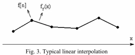
3. Linear Interpolation: In some cases f n[ ] does not have an equivalent function in the real domain with the same formula. For example,

1 k [ ] n ( 1) /k f n=

∑

− k

=

. In these cases we can find f xr( ) by interpolating f n[ ]

on real points. In linear interpolation we connect successive points of f[n] by a line. This method is very simple and has some useful properties.

Fig. 3. Typical linear interpolation

In the interval [ ,n n+1], f xr( ) can be found by the following formula: ( ) ( [ 1] [ ])( ) [ ] r

f x = f n+ −f n x n− + f n

To apply theorem 1 we have:

( ) ( 1) ( [ 1] 2 [ ] [ 1])( ) [ ] [ 1] , 1

[ ] [ 1]

[ 1] 2 [ ] [ 1] 0 [ 1] 2 [ ] [ 1]

( ) ( 1) 0

[ ] [ 1] 0

r r

r r

f x f x f n f n f n x n f n f n n x n f n f n

x n if f n f n f n

f n f n f n f x f x

f n f n otherwise

− − = + − + − − + − − ≤ ≤ +

− −

⎧ = − + + − + − ≠

⎪ _{+ − + −}

− _{− = ⇔ ⎨}

⎪ _{− − =}

⎩

Since n x n≤ ≤ +1 we have:

[ ] [ 1]

0 1 [ 1] 2 [

[ 1] 2 [ ] [ 1]

( ) ( 1) 0

[ ] [ 1] 0

r r

f n f n

if f n f n f n f n f n f n

f x f x

f n f n otherwise

− −

⎧

] [ 1] 0

≤ − ≤ + − +

⎪ _{+ − + −}

− _{− = ⇔ ⎨}

⎪ _{− − =}

⎩

− ≠

(3)

Lemma: _n* is a local minimum or maximum of the discrete function _{f n[ ]} if and only if:

* *

* * *

*

* *

[ ] [ 1]

0 1 [ 1] 2 [

[ 1] 2 [ ] [ 1] [ ] [ 1] 0

f n f n _{if f n f n f n}

f n f n f n

f n f n otherwise

⎧ − −

≤ − ≤ + − + − ≠

⎪ _{+ − + −}

⎨

⎪ _{− − =}

⎩

] [ 1] 0

(4)

Proof: Using (3) in theorem 1 it ends up at (4). Since in linear interpolation is monotonic for all

intervals for which m is an integer number, theorem 1 gives a necessary and sufficient

condition. In the cases that the solution of

( ) r f x ( ,m m+1)

( ) ( 1) 0 r r

f x −f x− = is integer, we have ,

which satisfies both parts of (4).

* *

[ ] [ 1] 0

f n − f n − =

Example 4: Find local minima and maxima of

1 ( 1) [ ]

k n k f n

k

= −

Using the lemma we have:

( 1) [ ] [ 1]

n f n f n

n

−

− − =

1 ( 1) [ ] [ 1]

0 1 0

[ 1] 2 [ ] [ 1] ( 1) ( 1)

1 1

0 1 0 0

2 1

n

n n

f n f n _n

f n f n f n

n n

n

and n n n

+ −

− −

≤ − ≤ ⇒ ≤ − ≤

+ − + − − −

− + +

⇒ ≤ ≤ ≠ ⇒ >

+

1

Thus, for every n>0, f n[ ]has a local minimum or maximum. Since [ ] [ 1] ( 1)

n f n f n

n

−

− − = , the even n’s

are local maxima and the odd ’s are local minima. n

Example 5: Find local minima and maxima of f n[ ] ( )= a n=a a( +1)...(a n+ −1).

Using the lemma we have:

[ ] [ 1]

0 1

[ 1] 2 [ ] [ 1] f n f n

f n f n f n

− −

≤ − ≤

+ − + −

2

( 1)...( 3)( 2)

0 1

( 1)...( 3)( 2){( )( 1) 2( 1) 1}

a a a n a n

a a a n a n a n a n a n

+ + − + −

≤ − ≤

+ + − + − + + − − + − +

Thus, each local minima or maxima of f n[ ] as should satisfy one of the following relations: _n*

* * 2

*

* *

( 1)...( 3)( 2) 0

or

( 2)

0 1

( 1)( 2) 1

a a a n a n

a n a n a n

+ + − + − =

+ −

≤ − ≤

+ − + − +

The solutions will simply be found by solving the above equality and inequality.

b) Multidimensional Discrete Optimization

Definition of local minimum and maximum for discrete multidimensional functions:

We say the vector ( , *,..., *)

2 *

1 k

* _{n n n}

n = is a local minimum of k-dimensional discrete function

with the domain if for all we have:

] ,..., , [n1 n2 nk f

f

D 1≤i≤k

{

{

1 2

1 2 '

1 2 '

( )

( 1 )

( 1 )

[ ] [ ] and

[ ] [ ]

* * * * k f

* * * * *

i k

i

i th element

* * * * *

i k

i

i th element

* *

i

* *

i

n n , n , ..., n D ,

n n , n , ..., n , ..., n D ,

n n , n , ..., n , ..., n D ,

f n f n

f n f n .

+

−

+

−

= ∈

= +

= −

≥ ≥

f f

∈

∈

i.e. *

n in all dimensions of f[n1,n2,...,nk] should be a local minimum.

We say the vector ( , *,..., *)

2 *

1 k

*

n n n

n = is a local maximum of k-dimensional discrete function

with the domain if for all we have:

] ,..., , [n1 n2 nk f

f

. n f n f

n f n f

, D , ..., n n

, ..., , n n n

, D , ..., n n

, ..., , n n n

, D , ..., n , n n n

* *

i

* *

i

f * k element th i

* i * * * i

f * k element th i

* i * * * i

f * k * * *

] [ ] [

and ] [ ] [

) 1 (

) 1 (

) (

' 2 1

' 2 1

2 1

≤ ≤

∈ −

=

∈ +

=

∈ =

− + − +

3 2 1

3 2 1

i.e. *

n in all dimensions of f[n1,n2,...,nk] should be a local maximum.

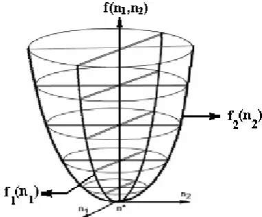
Thus, to find the local minima and maxima of a discrete multidimensional function we can apply theorem 1 to each of its dimensions, if it is feasible. A simple visualization of the above discussion is illustrated in Fig. 4 where theorem 1 has been applied to each of its dimensions. In theorem 2 we elaborate on this subject.

Fig. 4. n* is minimum of f(n1,n2)and in the dimensions n1 and n2 , n1* and n2*

are minima of f1(n1) and f2(n2) respectively

Theorem 2:

Suppose that f[n1,n2,...,nk] is a k-dimensional discrete function defined on

k

Z

D

⊂

and is

a continuous k-dimensional real function defined on so that , and at each integer point

such as

) ,..., , ( 1 2 k r x x x f

k r

R

D

⊂

D

⊂

D

_r

) ' ,..., ' , ' (

' n1 n2 nk

n= we have ( )f n_r ′ = f n[ ]′ . Consider the following k equations:

k i 1 ; 0 ) ,..., 1 ,..., ( ) ,..., ,...,

( 1 i k − r 1 i− k = ≤ ≤

r x x x f x x x

f (5)

If in the ith equation we can explicitly express in terms of other ’sx_i xj , (j≠i) for all , i.e. if we

can write the above equations in the following form (in which is a function of all ’s except ):

k i≤ ≤

1

(.)

i

g

xj xi

1 1 2

2 2 1

1 1

( ,..., )

( ,..., )

( ,...,

)

k k

k k k

x

g x

x

x

g x

x

x

g x

x

₋

=

=

=

M

(6)

Then using the functions

g

_i

(.)

in (6) and changing variables

x x

₁

, ,...,

₂

x

_k to integer variables ,

we create the following system of k equations:

1 1 2

2 1 1

1 1

[ ( ,..., )]

[ ( ,..., )]

[ ( ,...,

)]

k k

k k k

n

g n

n

n

g n

n

n

g n

n

₋

=

=

=

M

(7)

Where

[

g

_i

(.)]

denotes the integer part of

g

_i

(.)

.

Let

N N

₁

,

₂

,...,

N

_m be all the solutions of the above system of k equations. Where:

1 2 k j= 1j 2j k j , 1, 2

j , ... ,

N =(n ,n ,...,n ) (n ,n ,...,n ) j= m

(note that n_ij’s are integer since in the equation

n

_i

=

[ ( ,..., )]

g n

_{i 1}

n

_k , should be integer). n_i

If the set Ak consists of all Nj’s plus all the vectors

{

1 '

..., 1 i

j j ij kj

i th element

N =(n , n − ,...,n ) , (1≤j≤m, 1≤i≤k)

for which g N_i( _j) is an integer number (where g N_i( _j)=g n ,n ,... n_i( _{1j 2j} , ,..._lj ,n_kj) and

l

), then the set

i

≠

k

A contains all localmaxima and minima of f[n1,n2,...,nk].

Proof:

Let the vector be a local minimum of the function . According to the definition

of local minimum for discrete multidimensional functions for all

) ,..., , ( * * 2 *

1 n nk

n f[n1,n2,...,nk]

k i≤ ≤

1 we have:

]. ,..., , [ )] ,..., 1 ,..., , [( and ] ,..., , [ )] ,..., 1 ,..., , [( * * 2 * 1 * * * 2 * 1 * * 2 * 1 * * * 2 * 1 k k i k k i n n n f n n n n f n n n f n n n n f ≥ − ≥ +

This means that is a local minimum for the discrete one-dimensional function: *

i n ] ,..., ,..., [ ] [ * *

1 i k

i f n n n n

f = (1≤i≤k)

In which only is variable. According to theorem 1 the equation: ni

* * * *

1 1

( ,..., ,..., ) ( ,..., 1,..., ) 0 ,1 i k

r i k r i k

f n x n −f n x − n = ≤ ≤ (8)

has at least one solution for in the interval . If we can write the Eqs. (5) in the form of Eqs.

6), then we can also write the Eqs. (8) in the form:

i

x [ *, *₊1]

i i n n

(

* * 1 1 2

* * 2 2 1

* * 1 1 ( ,..., ) ( ,..., ) ( ,..., ) k k

k k k

x g n n

x g n n

x g n n ₋

= =

=

M

Thus, * *

1

( ,..., )

i i k

x =g n n would be the unique solution of the equation * * * *

1 1

( ,..., ,..., ) ( ,..., 1,..., ) 0

r i k r i k

f n x n − f n x − n = .

Thus, according to theorem 1, xi =g ni( ,..., )₁* n*k is in the interval . If all the ’s for

are in the interval , the integer parts of ’s would be equal to . In

this case, the solutions of the system of k Eqs. (7) contain . If some of the ’s are

equal to (which is integer), solutions of the system of k Eqs. (7) contain

for and both and would be in the set

] 1 , [ * *₊ i i n

n g ni( ,..., )₁* nk* 1 2i= , , …, k [ *, *₊1)

i i n

n g n_i( ,..., )₁* n*_k *

i n ) ,..., , ( * * 2 *

1 n nk

n g n_i( ,..., )₁* n*_k 1

*₊ i

n ( *,..., * 1,..., *)

1 ni nk

n +

1 2i= , , …, k ( *,..., * 1,..., *)

1 ni nk

n + ( *,..., *,..., *)

1 ni nk

n A_k.

In each case the set A_k contains ( *,..., *,..., *). Thus the set

1 ni nk

n A_k always contains all local minima of

. Similarly, using theorem 1 we can show that the set

] ,..., , [n1 n2 nk

f A_k always contains all local maxima

Note: When the discrete function is given by a mathematical formula we can use the same

formula for by substituting the discrete variables with the real variables

whenever the resulting is a continuous function. For example, if

we can choose

] ,..., , [n1 n2 nk f

) ,..., , ( 1 2 k r x x x

f n1,n2,...,nk

k x x

x1, 2,..., fr(x1,x2,...,xk) 2

2 1 2

1, ] ( )

[n n n n

f = + 2

1 2 1 2

( , ) ( )

r

f x x = x +x . We use the notation:

1 2 1 1

,

( [ , ,..., ]) ( ,..., ,..., ) ( ,..., 1,..., )

r

k r i k r i

i f

dif f n n n = f x x x −f x x − x_k

When has the same formula as , we drop the index in the above notation

and use the notation:

) ,..., , ( 1 2 k r x x x

f f[n1,n2,...,nk] fr

1 2 1 1

( [ , ,..., ])_k ( ,..., ,..., )_{i k} ( ,..., _i 1,..., )

i

dif f n n n = f x x x −f x x − x_k

Example 6:

In an industry there are some workers in k different units. The wage of each worker in the ith unit is $

per day and the per day income of the ith unit is given by , where is the number of workers

and

i

C

(1 2 )ni

i A ₋ −

i n i

A shows the maximum accessible income for the ith unit. We would like to obtain the optimal

number of workers in each unit in order to maximize the total profit of the industry. We assume that

for 1, 2,..., i i

A ≥C i= k

i i

. This means that the maximum income of each unit must be at least equal to the wage of one worker in that unit; a necessary condition to keep the unit profitable, otherwise the unit will not be operative even with one worker.

The total profit of the industry can be computed by:

1 2

1 1

[ , ,..., ] (1 2 )i

k k

n

k i

i i

f n n n A − C n

= =

=

∑

− −

∑

We have:

1 2

1 1

( , ,..., ) (1 2 )i

k k

x

k i

i i

i i

f x x x A − C x

= =

=

∑

− −

∑

Applying theorem 2 we have:

1 2

( [ , ,..., ]) 0

_k

1, 2,...,

i

dif f n n

n

=

i

=

k

Using properties 1 to 3 of operator dif we have:

1 1 2

2 2

( [ , ,..., ]) 2 2 0

2 ( 1 2) 2

log ( ) log ( )

i i

i i

x x

k i i i

i

x x i

i i

i

i i

i

i i

dif f n n n A A C

C

A C

A

C A

x

A C

− − +

− −

= − + − =

⇒ − + = ⇒ =

⇒ = − =

According to theorem 2 the optimal value for can be obtained as: n_i

2 2

*

2

2 2

[log ( )] if log ( ) is noninteger

log ( ) and

log ( ) 1 if log ( ) is integer

1,2,...,

i i

i i

i i

i

i i

i i

A A

C C

A n

C

A A

C C

i k

⎧ ⎪ ⎪ ⎪ = ⎨ ⎪ ⎪

− ⎪

⎩ =

(9)

2

2

1 log 0

[log ] 0

i i

i i

i i

A A

C C

A C

≥ ⇒ ≥

⇒ ≥

Thus, the optimal number of workers is always nonnegative and (9) is always valid. Note that in the case

of havinglog2 i 0

i A

C = and log2 1 1

i i A

C − = − , only log2 0

i i A

C = would be a valid optimal solution for . ni

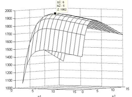
The computer simulation confirms the validity of this result. Figure 5 shows the profit of the industry

versus n1 and n2 in the case that k=2, A1=1000, A2=1200, C1=10 and C2=25.

According to this simulation the optimal values for n1 and n2 are 6 and 5, respectively. This result agrees

with the result obtained in (9).

Fig. 5. Profit of the industry versus n1 and n2 with k=2, A1=1000, A2=1200, C1=10 and C2=25. It is

obvious that the optimal values for n1 and n2 are 6 and 5, respectively.

Example 7:

Find local maxima of the joint probability mass function of the discrete normal random variables, , given by:

1

, ,...,

2 k

n n

n

( ( 1 2

[ , ,..., ] T_S

k

P n n n ₌ae−N - )μ N - )μ

where [ , ,..., ]_{1 2} Tis the vector of integer random variables,

k

N = n n n

[ , ,..., ]

1 2

T k

μ

=

μ μ

μ

is the mean vector

of N, a is a scalar positive constant and S is a

k k

×

constant matrix (inverse of covariance matrix of N).

We can minimize (_N−μ)T_{S N}( _{−μ) instead of maximizing} (_N )T_{S N}(

ae− −μ −μ)_{. Then we have:}

1 2

1 1 1

1 1

1 1

( ) ( )

[ ( ) ( ) ... ( )]( )

( ) ( )

( )( )

T

k k k

i i i i i i ik i i

i i i

k k

j j ij i i

j i

k k

ij i i j j

j i

N S N

S n S n S n N

n S n

S n n

μ μ

μ μ μ

μ μ

μ μ

= = =

= = = =

− − =

− − −

= − −

= − −

∑

∑

∑

∑

∑

∑∑

μ −

Let x x₁, ,...,₂ x_k be real variables and [ , ,..., ]1 2

T k X = x x x .

1 1

( )T ( ) k k ( )(

ij i i j j

j i

X μ S X μ S x μ x )

= =

)

(( ) ( ))

( ) ( ) ( ) (

T

l

l l

T T

dif N S N

X S X X S X

μ μ

μ μ μ

− − =

− − − − −μ

where l [ ,...,₁ 1,..., ]T

l k

X = x x − x .

Only the terms that contain

x

_l remain and the other terms vanish:

1 1

1 1

2 2

1 1

(( ) ( ))

( )( ) ( 1 )( )

( )( ) ( )( 1 )

( ) ( 1 )

( ) ( ) 2 (

T l

k k

lj l l j j lj l l j j

j j

j l j l

k k

il i i l l il i i l l

i i

i l i l

ll l l ll l l

k k

lj j j il i i ll l

j i

j l i l dif N S N

S x x S x x

S x x S x x

S x S x

S x S x S x

μ μ

μ μ μ μ

μ μ μ μ

μ μ

μ μ μ

= =

≠ ≠

= =

≠ ≠

= =

≠ ≠

− − =

− − − − − −

− − − − − −

+ − − − −

= − + − + −

∑

∑

∑

∑

∑

∑

_l)−S_ll

+

Combining the two summations in one yields:

1

1

(( ) ( )) ( )( ) 2 ( )

(( ) ( )) 0

1

( )( )

2 2

= ≠

= ≠

− − = + − + −

− − =

+

⇒ = + − −

∑

∑

k T

lj jl j j ll l l ll

l j

j l T

l

k

lj jl

l l j j

j _ll j l

dif N S N S S x S x S

dif N S N

S S

x x

S

μ μ μ μ

μ μ

μ μ

−

)

(10)

According to theorem 2 and considering only one of the solutions for the case of getting successive equal

minima, the minima of (_N−μ)T_{S N}( _{−μ satisfy the following system of k equations:}

* *

1 1

[ ( )( )]

2 2

1,...,

k

lj jl

l l j j

j _ll

j l

S S

n n

S

l k

μ μ

= ≠

+

= + − −

=

∑

(11)

Where (11) is obtained by changing real variables in (10) to discrete ones and taking integer part. denotes optimum value for . If is integer, then

* l n

l

n n_l * ₁

l

n − may also be a solution for . n_l

If S 1₂ I

σ

= we have:

* _[ 1_{] , 1,...}

2

l l

n = μ + l= ,k

I )

(12)

Where in (11) and (12), [.] denotes the integer part function.

For k=2 and _μ=[7.6 12.3]T, if _S=0.1 , according to (12), the maximum of (_N )T_{S N}(

ae− −μ −μ _{occurs at}

. If , substituting the parameters in (11) we have:

* *

1

8 ,

2

12

n

=

n

=

0.1 0.05

0.05 0.1

S_{= ⎢}⎡ − ⎤

−

⎣ ⎦⎥

* *

1 2

* *

2 1

1

[1.95 ]

2 1

[9 ]

2

n n

n n

= +

)

Only * * satisfy the above equations, thus it is the maximum of

1

7 ,

2

12

n

=

n

=

(_N )T_{S N}(

ae− −μ −μ _{. Although in}

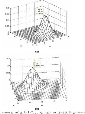
these two examples the mean vectors are the same, the maxima are different. Computer simulations

confirm these results. Figure 6 shows (_N )T_{S N}(

ae− −μ −μ)

versus

n

₁ and

n

₂ for the above cases.

(a)

(b) Fig. 6. a) (_N )T_{S N}( )

ae− −μ −μ versus and for k=2,

1

n n2 μ=[7.6 12.3]T, and S=0.1I, b) ( ) ( ) T

N S N

ae− −μ −μ versus

1

n

and n₂ for k=2, _μ=[7.6 12.3]T, and 0.1 0.05 0.05 0.1

S_{= ⎢}⎡ − ⎤_⎥

−

⎣ ⎦

3. CONCLUSION

A novel analytical approach has been presented for the first time to solve multidimensional and multimodal discrete optimization problems. This approach has complete preference over the existing methods. In this approach the local minima and maxima of discrete functions can be evaluated by analytical formulas that enormously reduce the complexity of computations. All the existing methods have been developed based on algorithmic approaches such as integer programming (IP) and exhaustive search method that are very complex, need a high order of computations, and usually lead to suboptimal algorithms.

REFERENCES

3. Li, D. & Sun, X. L. (2006). Nonlinear integer programming. Springer.

4. Nowak, I. (2005). Relaxation and decomposition methods for mixed integer nonlinear programming. Birkhäuser, Basel.

5. Karlof, J. K. (2005). Integer programming: theory and practice. CRC.

6. Appa, G., Pitsoulis, L. & Williams, H. P. (2006). Handbook on modeling for discrete optimization. New York, Springer.

7. Tuy, H., Minoux, M. & Hoai-Phuong, N. T. (2006). Discrete monotonic optimization with application to a discrete location problem. SIAM Journal on Optimization. Vol. 17, No. 1, pp. 78–97.

8. Poljak, S. (1995). Integer linear programs and local search for max-cut. SIAM Journal on Computing, Vol. 24, No. 4, pp. 822-839.

9. Liu, M. & Ubhaya, V. A. (1997). Integer isotone optimization. SIAM Journal on Optimization, Vol. 7, No. 4, pp. 1152-1159.

10. Zimmermann, U. (1990). Review of discrete optimization (R. G. Parker and R. L. Rardin). SIAM Review, Vol. 32, No. 2, pp. 333-334.

11. Blair, C. (1990). Review of integer and combinatorial optimization (G. L. Nemhauser and L. A. Wolsey). SIAM Review, Vol. 32, No. 2, p. 315.

12. Seyed-Hosseini, S. M. & Jenab, K. (2004). The development of the tabu search technique for expansion policy of power plant centers over specific defined reliability in long range planning. Iranian Journal of Science and Technology, Transaction B, Engineering, Vol. 28, No. B2, pp. 217-224.