QUEST FOR ROBUST OPTIMAL
MACROPRUDENTIAL POLICY
Pablo Aguilar, Stephan Fahr, Eddie Gerba
and Samuel Hurtado
Documentos de Trabajo
N.º 1916
QUEST FOR ROBUST OPTIMAL MACROPRUDENTIAL POLICY (*)
Pablo Aguilar and Samuel Hurtado
BANCO DE ESPAÑA
Stephan Fahr
EUROPEAN CENTRAL BANK
Eddie Gerba
DANMARKS NATIONALBANK
Documentos de Trabajo. N.º 1916 2019
The Working Paper Series seeks to disseminate original research in economics and fi nance. All papers have been anonymously refereed. By publishing these papers, the Banco de España aims to contribute to economic analysis and, in particular, to knowledge of the Spanish economy and its international environment.
The opinions and analyses in the Working Paper Series are the responsibility of the authors and, therefore, do not necessarily coincide with those of the Banco de España or the Eurosystem.
The Banco de España disseminates its main reports and most of its publications via the Internet at the following website: http://www.bde.es.
Reproduction for educational and non-commercial purposes is permitted provided that the source is acknowledged.
Abstract
This paper contributes by providing a new approach to study optimal macroprudential policies based on economy wide welfare. Following Gerba (2017), we pin down a welfare function based on a fi rst-and second order approximation of the aggregate utility in the economy and use it to determine the merits of different macroprudential rules for Euro Area. With the aim to test this framework, we apply it to the model of Clerc et al. (2015). We fi nd that the optimal level of capital is 15.6 percent, or 2.4 percentage points higher than the 2001-2015 value. Optimal capital reduces signifi cantly the volatility of the economy while increasing somewhat the total level of welfare in steady state, even with a time-invariant instrument. Expressed differently, bank default rates would have been 3.5 percentage points lower while credit and GDP 5% and 0.8% higher had optimal capital level been in place during the 2011-2013 crisis. Further, using a model-consistent loss function, we fi nd that the optimal Countercyclical Capital Buffer (CCyB) rule depends on whether observed or optimal capital levels are already in place. Conditional on optimal capital level, optimal CCyB rule should respond to movements in total credit and mortgage lending spreads. Gains in welfare from optimal combination of instruments is higher than the sum of their individual effects due to synergies and positive mutual spillovers.
Keywords:optimal policy, global welfare analysis, fi nancial stability, fi nancial DSGE model, macroprudential policy.
Resumen
Este artículo propone una nueva aproximación al análisis de las políticas macroprudenciales basado en el bienestar de la economía. En línea con Gerba (2017), fi jamos una función de bienestar con criterios de primer y segundo orden ligados a la utilidad agregada de la economía para determinar los benefi cios de distintas reglas macroprudenciales en la zona del euro. Esta propuesta es evaluada en el marco del modelo de Crec et al. (2015). Los resultados muestran que el nivel de capital óptimo es de un 15,6 %, 2,4 puntos porcentuales por encima de la media del período 2001-2015. Situándose los requisitos de capital en su nivel óptimo se reduce signifi cativamente la volatilidad de la economía, a la vez que aumenta el nivel de bienestar a largo plazo, aun siendo un instrumento invariante en el tiempo. Dicho de otro modo, bajo el nivel óptimo de capital el porcentaje de quiebras bancarias hubiera sido 3,5 puntos porcentuales menor, y el crédito y el PIB, un 5 % y un 0,8 % mayores respectivamente, durante la crisis de 2011-2013. Además, con el uso de una función de pérdidas consistente con el modelo, encontramos que la regla para el colchón de capital contracíclico (CCyB) depende de si la economía se encuentra en su nivel óptimo de capital o no. Condicionado a esto último, los resultados sugieren que el CCyB óptimo debe responder a movimientos en el crédito y en los diferenciales hipotecarios. Además, las ganancias en términos de bienestar resultan mayores cuando la determinación de ambas herramientas macroprudenciales es conjunta gracias a las sinergias que se generan.
Palabras clave:política macroprudencial óptima, análisis de bienestar, estabilidad fi nanciera,
modelos de equilibrio general.
1Analogous to a Taylor rule for monetary policy, this instrument responds to cyclical deviations in certain variables, and its ability to influence the economy should be in the short- and medium-run only.
Following the Great Financial Crisis (GFC) in 2008, a set of macroprudential
tools have been designed and implemented to contain and reduce systemic risks,
increase the soundness of the financial system, and prevent a repetition of the sharp
reversal observed in 2007-08. Capital-based measures currently represent the
cor-nerstone of the macroprudential toolkit, and because of that several academic
pa-pers have assessed the impact of adjusting capital requirements on the resilience of
the banking sector and costs to banks in terms of financing costs, external financing
spreads, credit supply, and financing flexibility. While important and relevant, those
studies often take a reduced-form view on the costs and benefits, and allow a lot of
space for subjective evaluation of net benefits.
This paper takes a different approach and examines the net benefits from a
comprehensive and systematic viewpoint. Recognising that these measures have
both benefits and costs, the approach taken here weights these in an objective and
model-consistent manner, and evaluates net benefits for the totality of the economy.
In particular, we take the method developed in the monetary policy literature on
optimal rules (see for example Woodford (2003) or Gali and Monacelli (2004)), and
adapt it to the particularities of macroprudential policy.
This paper builds on this literature by providing analytical, model-consistent
and easily quantifiable welfare criteria that are then used to derive optimal
macro-prudential policies. First we analytically derive a second-order welfare criterion that
incorporates both long-run level and shorter-run volatility effects, and use it to find
the optimal level of capital requirements. Next, we derive a loss function that only
includes second order terms, and use it to search for an optimal countercyclical
buffer (CCyB) rule.1 The third and final section examines the interaction between
these two capital-based measures, and finds that the shape of the optimal CCyB
rule changes depending on whether the capital requirement has already been set
to its optimal level. Together with the finding that suboptimal specifications or
parameters can easily lead to welfare losses relative to inaction, this is an indication
that CCyB rules are more difficult to implement, since the optimal specification and
parameters depend on whether other policies have already been implemented. To
test its’ performance, the method is applied to the medium-scale financial DSGE
model of Clerc et al (2015) involving six types of agents, where three of them can
endogenously default (banks, borrower households, and entrepreneurs).
The paper is particularly relevant for policy-makers since it provides a novel
macro-prudential measures. Moreover, it provides a framework that allows regulators to
compare and assess, in terms of welfare losses, how close or far away the current
implemented measures are from that optimum level. In some cases, because
wel-fare is not observable, policymakers may prefer to use quantifiable variables such as
GDP, credit, or probability of crisis in order to measure the effects of implemented
macropudential policy instruments; this framework is flexible enough to compare
these alternative instruments to the optimal. Finally, counterfactual scenarios can
be simulated (and we do so in this paper) to show the economic performance that
would have materialized had optimal instruments been activated in the first place.
Our main results are: First, the optimal level of risk-weighted capital for Euro
Area is 15.6 percent. This is 2.4 percentage points higher than the average level
ob-served during the 2001-2015 period. And we find that setting the capital level ’too
high’ is more forgiving than setting it ’too low’: while the welfare is only marginally
reduced when deviating to the right of the optimal level (overshooting), the
reduc-tion in welfare is much higher when deviating to the left (undershooting). This is
important because in real time the policy-maker will always hold imperfect
informa-tion regarding the contemporaneous economic structure and shocks. Second, the
optimal EA CCyB rule is one that responds to developments in total credit and house
prices. However, this result rests on the premise that the exact weights in the rule
are implemented since the area of admissible coefficients is very narroiw. In other
words, weight misspecification can generate significant welfare costs and so great
attention should be placed in applying the exact optimal weights. Third, once an
optimal capital level has been implemented, the range of permissible weights in the
CCyB rule that expands, which reduces the probability of misspecifying the CCyB,
making it more robust. In addition, the optimal CCyB rule changes to one that
responds to total credit and mortgage lending spreads. Also global welfare is in this
case considerably higher compared to the sum of welfare gains that the two optimal
policies generate separately. This means that one optimal policy exerts positive
ex-ternalities on the other and generate positive synergies, which results in higher joint
gains. Fourth and final, we show that, according to the model, credit and GDP
losses since the GFC would have been significantly smaller (between 7 and 13 % for
credit and 1.25% for GDP) and the default probability of banks could have been
greatly reduced (by up to 3.6 percentage points), had the authorities implemented
the optimal combination of capital-based instruments in the first place.
The rest of the paper is organised as follows. Section 1 provides a conceptual
discussion on the role of macroprudential policy using existing literature and
some key distortions it attempts to correct. Section 2 discusses the optimal level of
capital by first deriving a model-implied and utility-based optimality criterion and
then testing it within this particular framework. We also compare it to alternative
simpler criteria popular in policy circles. Section 3 considers optimality criteria for
the setting of optimal countercyclical buffers and searches for specific examples.
Sec-tion 4 discusses the interacSec-tion between the optimal level of capital and the optimal
CCyB rules. Lastly, section 5 concludes.
1
The role of macroprudential policy
Literature on macroprudential policy is relatively new but quickly growing. The
main challenge has been to provide the fundamental building blocks to accommodate
for a system-wide financial policy in a general equilibrium framework. The current
debate can be synthesized under two streams, where (at the moment), the first one
has been discussed and used more widely to motivate the need for a system-wide
financial intervention.
The first line of research focuses on the negative pecuniary externalities that
financial contracts, financial decisions and interactions between banks cause because
they do not take into account the wider (or later) impact of their actions on the
financial system, or the economy (Davila and Korinek (2017)). De Nicolo, Favara
and Ratnovski (2012) categorize these externalities into three types: externalities
related to strategic complementarities, externalities related to interconnectedness,
and externalities related to fire sales. The first type arises as a result of strategic
interactions between financial intermediaries and may lead to a build-up in
system-wide vulnerabilities, in particular during a financial boom. The second variety of
externality arises as a result of the tight and complex network that exists between
financial actors, which can easily propagate (small) negative shocks throughout the
entire system. The third type is caused by a broad sell-off in assets during financial
downturns, which leads to a heavy drop in asset prices and balance sheets of financial
intermediaries. Following from these distortions, Mendoza (2016 and Bianchi and
Mendoza (2018) show how macroprudential tools such as value or
loan-to-income ratios can, much like taxes, correct for them and internalize (at least) some
of these externalities.
The second research stream focuses on the aggregate demand externalities that
agents exercise on others when signing financial contracts. Ex ante, agents do not
take into account the externalities their asset positions have on aggregate demand in
lower bound) this distortion can have quantitatively large effects on future demand,
and the general equilibrium becomes constrained inefficient. Fahri and Werning
(2016) provide an exact way to calculate this externality as well as the tax that is
required to correct for it. This tax can, from an ex ante point of view, be viewed
as a macroprudential tool since it incentivizes or penalizes particular behaviour or
contracts.
Despite their differences in type of distortions and channels, the role of
macro-prudential policy is akin to that of fiscal policy in both streams. The rationale for
the use of policy is very similar to that of Pigouvian taxes, and they generate high
redistributive effects. While in practice that is easy to relate with borrower-based
measures such as loan-to-value/income, debt-to-value/income, or even
total-debt-service-ratio, the link to capital-based measures is not as straight-forward. In
par-ticular, capital-based tools do not directly affect the income or value of borrowers,
but has rather an impact on the decision and quantity of loans supplied, as well
as the willingness of savers to deposit. The key variable that these measures are
(preventivly) aiming at minimizing is the expected probability of default of banks.
As shown in the previous section, capital requirements aim at keeping this
proba-bility as low as possible such that the default event never materializes at any point
in the future. However, since risks build up over the cycle, additional measures
need to be employed in order to tackle these cyclical hazards, which in turn may
in-crease the overall default probability. For that, CCyB is especially tailored to take
into account these time-varying risks. Albeit these measures do not restrain the
borrowers’ fiscal position directly, indirectly they do by determining their liquidity
(money) holdings, which has some redistributive effects. Moreover, at the heart of
the financial dynamics (and the default probability) is the bank’s incentive to lever
up and overextend credit from a social perspective. Taking this into account, the
motivation for macroprudential policy in this model seems to be closer to that of the
first strand, in particular to the externalities related to strategic complementarities.2
1.1
Motivation for macroprudential policy
The best way to test a method is to apply it to a specific framework. For this
pur-pose, we have chosen the dynamic structural model of Clerc et al. (2015) because it
is constructed with Euro Area banking sector and financing specificities in mind as
well as because it provides an explicit rationale for capital regulation by introducing
two types of distortions: limited liability on the part of banks, and bank funding
cost externalities resulting in excessive risk-taking by banks. The model introduces
financial intermediaries and three layers of default into an otherwise standard
dy-namic stochastic general equilibrium (DSGE) framework, but absent nominal and
real rigidities. While in this model defaults can occur among banks, non-financial
corporations and households, the key default that triggers macroprudential policy
is that of banks.
The model includes six types of representative agents: borrowers, savers,
en-trepreneurs, banks, bankers, and the macroprudential authority. However, because
the focus of the model is on financial relations, the majority of the dynamics is
con-centrated to the banking sector. Banks finance their loans by raising equity (from
bankers) and deposits (from savers). Deposits are formally insured by a deposit
insurance agency that is funded by lump-sum taxes paid by savers and borrowers.
When banks default (a non-linear event) depositors suffer some transaction costs
despite the deposit insurance scheme. This feature effectively links bank risk to
banks’ funding costs.3
However, banks’ cost of funding is not related to banks’ individual risk taking.
Instead, it is dependent on the system-wide risk pattern. This is due to two factors.
First, safety-net guarantees insulate banks’ cost of deposits from the effect of their
individual risk taking. Second, the deposit premium is based on system-wide bank
risk failure. This reduces the incentive of any individual bank to limit leverage and
failure risk because it will get no funding cost premia (benefit) when depositors are
assumed to be imperfectly informed.
Moreover, banks have an incentive to take as much risk as possible by leveraging
up to the regulatory limit. This excessive leverage has two counter-acting effects
on their funding costs in equilibrium. On one hand, default probability of banks
increases, which exerts upward pressure on banks’ funding costs. On the other,
this results in higher bailout subsidy (and taxes), which puts downward pressure on
their funding costs. The net effect depends on which of the two dominates. Ifoverall
bank failure risk is high, the first effect (higher deposit premium) dominates, and the
excessive leverage depresses economic activity. Ifoverall bank risk is low, excessive
leverage will support economic activity. Economising on expensive equity reduces
overall bank funding costs, and higher leverage will increase economic activity.
Higher capital ratios tighten the supply of loans by reducing the incentives for
banks to take on excessive leverage. At the same time, higher capital ratios reduce
the cost of uninsured funds provided to banks, which in turn reduces the cost of
credit. The final impact depends on which of the two channels dominates. Moreover,
the heterogeneity in households means that there is a trade-off between the welfare of
savers and borrowers. In the long run,savers benefit from tighter capital regulation
due to the reduced likelihood of bank failures which implies safer bank deposits.
Borrowers, meanwhile, lose out after a certain level of capital, as this leads to a
reduced supply of loans. Because of these multiple trade-offs, the model is well-suited
to detect an optimal level (and combination) of policy since there is a well-identified
global welfare function. In addition, once the optimal policy has been identified,
it can be used to calculate the general equilibrium effects from such policy (mix),
as well as extract the precise gains (distance) from alternative scenarios (involving
alternative policy options or no policy at all). Our method is originally inspired
by the one used for optimal monetary policy (see Woodford (2003), De Fiore and
Tristani (2009), Gerba (2017) or Ferrero et al (2018), but with some important
modifications and adaptations to take into account the differences in objectives,
targets, and instruments used in macroprudential policy and financial stability.
1.2
Key mechanisms
The key mechanisms and trade-offs relevant to the welfare analysis are within the
banking sector. In the next few lines, we will proceed to describe the composition
of bank liabilities, as well as the regulatory requirements.
The aggregate default rate for the banking system,P Dtb, which is also the fraction
of deposits in banks that fail in period t is determined by:
P Dtb = d H
t−1P DHt +dFt−1P DFt
dHt−1+dFt−1 (1)
where P DtH is the default rate for borrowing households, P DFt that of firms,
dHt−1 is the share of deposits lent out to borrowing households, and dFt−1 the share lent out to entrepreneurs. The average default rate of banks is the weighted average
of the default rates of the creditors (borrowers and entrepreneurs). This rate, in
turn, determines the interest rate on deposits since savers demand a risk premium
on their deposits depending on the (average) default rate of banks according to:
˜
RDt =RDt−1+ (1−γP Dbt) (2)
Notice the time-dependency of the deposit rate, but in extreme cases (when
P Dtb is very high) it can become non-linear and significantly deviate from previous
periods deposit rate.
Note also that in this model, the probability of households’ default on their loans,
and an aggregate shock. Thus, the debt is not state-contingent, and loan and deposit
contracts are incomplete insofar that they can’t be made contingent on aggregate
variables., Thus, while the debt contract shields against idiosyncratic shocks, it is
directly affected the aggregate shock, throughRHt that is theex post average realized
gross return on housing:
RtH = q H
t (1−δtH
qtH−1 (3)
In turn, the deposits held by savers must equal the sum of the demand for deposit
funding from the banks making loans to households, dHt−1 = (1−φHt )(qtHhmt xet/Rmt ), and from the banks extending loans to entrepreneurs, dFt−1 = (1−φtF)(qtKkt−(1− χe)Wte), that is:
dt =dFt−1+dHt−1 ≡(1−φFt )(qtFkt−(1−χe)Wte) + (1−φHt )(qtHhmt xet/Rmt ) (4)
To continue with deposits, the losses caused by the failing borrowers and
en-trepreneurs are given by:
TtH =
¯
ωtH −ΓH( ¯ωHt ) +μHGH( ¯ωtH) ˜RHt q H
t−1hmt−1xet−1 Rtm−1
(5)
and
TtF =
¯
ωFt −ΓF( ¯ωtF) +μFGF( ¯ωtF) ˜RtFqtK−1kt−1(1−χe)Wte
(6)
that are covered with lump-sum taxes imposed on savers in order to fully cover
for the losses in each period Tt=TtH +TtF.
The other source of funding for banks, equity, is more costly and therefore
sup-plied in less quantity to banks. Total equity provided by bankers, n = (1−(1−
χe)Wtb) must equal the sum of the demand for bank equity for loans to borrowers,
eHt =φHt (qHt hmt xet/Rtm) and loans to entrepreneurs, eFt =φFt (qtKkt−(1−χe)Wte):
(1−χe)Wtb =φFt [(1−χe)Wte] +φHt q H
t−1hmt−1xet−1
Rmt−1 (7)
You will notice that, because equity is more expensive, the share of equity
fi-nancing, φt is minimal, and in steady state, just enough to cover the regulatory
capital requirements (since only equity can be used as eligible regulatory capital).
To conclude, we need to describe the characteristics and evolution of regulatory
capital. The total capital buffer, φjt consists of a structural (time-invariant) φ¯jo and
a cyclical component φ¯jt.
2
Optimal capital requirements
2.1
Optimality and global welfare function
It is not a priori clear whether the policy-maker wishes to impose a low or high capital
requirement. On one hand, high capital requirements lead to a low credit level, much
below the social optimum. On the other hand, a very low capital requirement may
lead to excessive bank leverage, which may take the entire economy into a default
state. Moreover, the effects may be non-linear with respect to different levels of
capital. Hence, the policy-maker (or social planner) should balance the two forces,
and take into account the fiscal costs involved in bank default.
The most comprehensive way to extract optimal bank capital levels is to subject
it to a welfare criterion that is global, model-consistent, and derived from the model’s
first principles. Only then can one genuinely speak of a vigorous optimal capital
ratio since that is the level that maximizes welfare of all consumers in the economy.
To find the criterion, we derive a first-and second order approximation of aggregate utility. Both household types are considered when constructing the aggregate utility
measure. The objective of the macroprudential authority is to find the capital level
that maximizes the level of (aggregate) utility while at the same time minimizing
the volatility of its’ arguments. That is why we capture both a first- (level) and
second order (volatility) term in the global welfare expression. The first order terms We call the second component a Countercyclical Capital Buffer (CCyB) that
depends on the state of the economy. We will in the subsequent sections discuss
what particular indicators of the (financial) cycle the rule should optimally respond
to. For the moment, we generally describe it as responding to deviations of a
number of (indicator) variables Σ from their trend (or steady state) values. In the
next section, we will also examine the optimal level of the structural component.
Note that the rule prescribes an additive approach to regulatory capital (in line with
Basel III), where the cyclical part is on top of the structural component, and not as
a substitute for it. Moreover, what we call here regulatory capital φjt is actually the
ratio of equity-to (risk weighted) assets. Therefore, this variable can also be written
as:
φjt = e F t +eHt (1−χe)Wte +
qtH−1hmt−1xet−1
Rmt−1 (9)
In the current model version, loans to borrowers (or borrowing households) has
a higher risk weight, and therefore will matter, in relative terms, more for the risk
E0
∞
i=0 βts+i
logcst+1+νsloghst+i−1− ϕ s
1 +η(l s t+i)1+η
(11)
for savers, and for borrowers:
E0
∞
i=0 βtm+i
logcmt+1+νmloghmt+i−1− ϕ m
1 +η(l m t+i)1+η
(12)
,whereβs > βm.
After derivations in Appendix I, we find that the above expression can be
ap-proximated and re-written to only include first-and second order additive terms
according to:
E0
∞
i=0
βt+i(Ut−U) =E0Σi∞=0βt+iWf +t.i.p+O3 (13)
with Wf =χhsμhs −χ2hsσh2s+χhmμhm−χ2hmσh2m+χwμw−χ2wσw2 +χkμk−χ2kσk2
where χhs ≡ζhνss − (1+Ihgh)−(1−δh),
χ2hs ≡ζνhss −(1+g h) Ih
−(1−δh),
χhm ≡(1−ζ)νhmm − (1+Ihgh)−(1−δh),
χ2hm ≡(1−ζ)ν m
hm − (1+g h) Ih
−(1−δh), χw ≡ (ϕs+ϕ1+mη)(1−α)ww
η2ss
2 ,
χw2 ≡ (ϕs+ϕ1+mη)(1−α), χk ≡ −1+Ig +δt,
and χ2k ≡ −1+Ig1Iδt+12l22δ.
are all added in order to collect all level-effects, while the second order terms are all
subtracted in order to subtract any changes in the volatility of the aggregate utility
following implementation of a policy. Because of the inherent trade-offs in banks’
lending activity, the welfare measure is expected to be hump-shaped with a (local
or global) maximum. In the following subsection, we will show the steps to derive
this function.
2.1.1 Deriving the utility-based welfare function
Households are the only consumers in our setting. Thus, the policy objective
func-tion will be a weighted average of the (approximate) utility funcfunc-tion of saver-and
borrower households, or:
E0
∞
i=0
βt+i[ζUts+ (1−ζ)Utm] (10)
where ζ is the weight of the utility of savers in the policy objective. The two utility
Using the calibrated values for the Euro Area explained in Clerc et al (2015),
and extracting the steady state values for the endogenous variables, we find the
following optimal weights for each of the arguments in the loss function:
χhs ≡3 (14)
χ2hs ≡3 (15)
χhm ≡3 (16)
χ2hm ≡3 (17)
χw ≡1.43 (18)
χ2w ≡0.05 (19)
χk ≡ −0.8 (20)
χ2k ≡0.005 (21)
Normalizing to 1 for χhm and χ2hm, the respective weights become:
χhs ≡ 3
3 = 1 (22)
χ2hs ≡ 3
3 = 1 (23)
χhm ≡ 3
3 = 1 (24)
χ2hm ≡ 3
3 = 1 (25)
χw ≡ 1.43
3 = 0.48 (26)
χ2w ≡ 0.05
3 = 0.02 (27)
χk≡ −0.8
3 =−0.27 (28)
χ2k≡ 0.005
This is the welfare function we use as objective criterion in our experiments to
find the optimal bank capital levels for Euro Area. Again, the optimal capital level
is the one that maximizes this objective function. The weights of each argument in
the welfare function are determined by the values in the calibration exercise for the
2001-14 period. If the calibrated values change, the weights will also change.
2.1.2 Alternative optimality criteria
An alternative to our approach would have been to compute directly the welfare
gains associated with any particular policy as a weighted average of the
consumption-equivalent gains of each household dynasty under the baseline policy (with capital
on firm loans twice as high as that on household loans) equal to the welfare under
alternative values of both capital ratios. The weight on each individual dynasty
is given by the share of that dynasty in aggregate consumption under the baseline
policy. The reported welfare gains would then be equal to:
ΔW ≡ c
s 0 cs0+cm0 Δ
s+ cm0 cs0+cm0 Δ
m (30)
c0 denotes the steady-state consumption of each dynasty under the baseline
pol-icy. While this measure is straight-forward (and hence why we compare our results
to it), it suffers from a number of drawbacks. First, the policy-maker does not
directly control agents’ consumption. Hence, his knowledge of the consumption
dy-namics is imperfect. Second, determining the share of each household dynasty (in
turn which dynasty matters more) becomes a subjective choice. Moreover,
deter-mining the share by the contribution of each to aggregate consumption under the
baseline policy is misguiding as this share may endogenously change due to
policy-makers undertaking alternative policies, as well as with the key policy parameters.
Third, the policy-maker would, in his welfare criterion, like to use variables that are
directly affected by default distortion and financial frictions. Fourth (and maybe
most important) consumer utility is determined by other factors besides
consump-tion. If one only considers consumption (levels and volatility), one may disregard
other factors that contribute to their total welfare.
For robustness purposes, we also compare our results to alternative ad hoc
ob-jective criteria that are often used (in practice) for determining the level of capital.
Examples of these criteria are: number of bank defaults, GDP losses, investment
losses, consumption losses, gains in utility of borrowers, or gains in utility of savers.
The aim is to contrast the capital levels prescribed by these criteria to our global
welfare criterion above, including a full comparison of the trade-offs and effects that
2.2
Quantitative results
2.2.1 Optimal capital level
In this section we evaluate the welfare gains with distinct levels of capital. In
other words, we are depicting the welfare function for a range of values of capital
requirements.
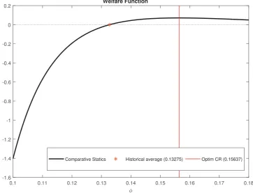
Graph 1 shows the percentage change in welfare relating to various capital levels
in relation to the level observed during the 2001-15 period. The historical average
level was 13.2%, while we compare it to capital levels ranging from 10 to 18%.
The graph shows that welfare initially improves quickly as we increase capital
levels, but that the rate of improvement drops once we approach the historical
av-erage. Nevertheless, it continues to increase even after that level, and reaches a
maximum at around 15.6%. At this level, the welfare is 10% higher compared to
the historical average. Since this is a (local) welfare maximum for reasonable levels
of capital, we consider 15.6% to be the optimal capital level for Euro Area. In
addi-tion, the shape of the welfare function suggests that, it is safer for macroprudential
authority toovershoot in setting the right capital level rather than undershoot. The
drop in welfare gains is significantly steeper to the left of the optimum compared to
the right of it. That means that the effects are indeed non-linear as capital levels
increase. Our welfare function can in a simple but holistic way capture them.
Al-though a bit more cumbersome, one can also view these asymmetric effects through
the individual macro-financial variables in the next figure. The percentage change
in the various variables at lower levels of capital and to the left of the optimum are
much higher then to the right, confirming this cost of ‘undershooting’.4
Putting these numbers into broader perspective will be helpful. In particular,
we wish to compare the broader economic (steady-state) effects that capital levels
from 10 to 18% have. At the same time, this allows us to contrast the general
equilibrium effects from the welfare criterion-based capital levels to those that would
be prescribed from more myopic or partial criteria such as the number of defaults of
banks or household consumption. This is also a more direct way to check whether
the welfare function-based optimum is as holistic as we claim and whether it succeeds
in balancing numerous trade-offs that are embedded within banks’ lending activity.
Figure 2 depicts these effects.
An increase in capital levels that takes them from their historical average to the
optimal value (an increase of approximately 2.4 p.p.) would make banks reduce
total credit to meet the capital requirements, but, given the difference in the risk
weight between corporate and commercial credit, the reduction would mainly affect
Euro Area - Comparative Statics wrt Capital requirement
0.1 0.11 0.12 0.13 0.14 0.15 0.16 0.17 0.18
-1.6 -1.4 -1.2 -1 -0.8 -0.6 -0.4 -0.2 0
0.2 Welfare Function
Comparative Statics Historical average (0.13275) Optim CR (0.15637)
Figure 1: Capital levels for Euro Area using the objective welfare function
corporate credit. At the optimal level of capital, banks become safer, with a
de-fault probability that is much closer to zero. The higher soundness of the financial
system reduces the insurance cost, and this generates an increase in consumption
and housing investment, whereas the reduction of corporate credit reduces business
Euro Area - Comparative Statics wrt Capital requirement
0.1 0.12 0.14 0.16 0.18
-1 0 1
% from historical average
GDP
0.1 0.12 0.14 0.16 0.18
-2 0 2
% from historical average
Household Consumption
0.1 0.12 0.14 0.16 0.18
-1 0 1
% from historical average
Business Investment
0.1 0.12 0.14 0.16 0.18
-5 0 5
% from historical average
Residential Investment
0.1 0.12 0.14 0.16 0.18
0 0.5 1
% annualized
Average Default Banks
0.1 0.12 0.14 0.16 0.18
-5 0 5
% annualized
Default NFC
0.1 0.12 0.14 0.16 0.18
-2 0 2
% annualized
Default HH
0.1 0.12 0.14 0.16 0.18
-10 0 10
% of GDP
Deposit Insurance Cost
0.1 0.12 0.14 0.16 0.18
-5 0 5
% from historical average
Total Credit
0.1 0.12 0.14 0.16 0.18
-2 0 2
% from historical average
NFC Loans
0.1 0.12 0.14 0.16 0.18
-10 0 10
% from historical average
HH Loans
0.1 0.12 0.14 0.16 0.18
3.2 3.4 3.6
% annualized
NFC Loan Rate
Comparative Statics Historical average (0.13275) Optim CR (0.15637)
2.2.2 Decomposition
To help understand the trade-offs involved in attaining the optimal level, the
fol-lowing figure decomposes the welfare function into its four components: the terms
associated to borrowers, savers, labor and (physical) capital (k) factors (always in
difference from the level each one has at the observed historical average). The
argu-ments in the welfare function have different shapes: the capital (k) factor is always
increasing in capital but small in comparison to the others, while the ones for wages,
borrowers and savers are all hump-shaped, but the latter in a different direction than
the first two.
The cases of borrowers and savers are interesting to discuss (and it is easier
to do so if we recall the comparative statics presented in Figure 2). When the
capital ratio is relatively low, an increase has a big effect in terms of reducing the
average default rate of banks, and this generates a decrease in financing costs for
all agents. Therefore in this range, even if the capital rate is increasing, total credit Figure 3: Decomposition of the welfare function across different capital levels and shocks
also grows, and the welfare of borrowers is increasing. Savers, on the other hand,
face both a lower interest rate and, at least initially, growing deposit insurance costs
(because, although banks’ average default rate is lower, total credit grows), so their
welfare is decreasing.5For high values of the capital ratio, the marginal reduction in
the average default rate of banks attained by a further increase becomes smaller:
the system is already very safe, and further increase in capital has bigger costs
than benefits. GDP, investment and credit are decreasing, and so is the welfare of
borrowers. Financing costs rise, as credit becomes scarcer, and this increases the
welfare of savers; this explains the fact that the social optimum is to the right of the
maximum of the welfare of borrowers, and in a range in which the argument related
to wages is clearly negative.
2.2.3 Counterfactual scenario
Apart from assessing the steady-state welfare effects of different levels of the capital
ratio, we can also run counterfactual scenarios to see how different macro variables
would have evolved in the 2001-2015 period if capital ratios had been different from
the beginning.
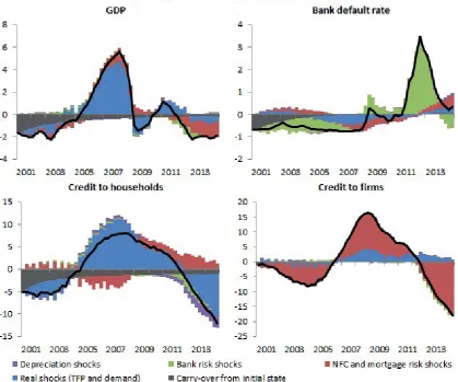
The first step for this is to use observed data (in detrended levels), the calibrated
model and the Kalman filter to construct a historical decomposition (in terms of
the structural shocks in the model) of the evolution of the main macro and banking
variables, in this case for the euro area in the period 2001-2014. The results in Figure
4 show that GDP and credit to households are driven mainly by real shocks, with
some relevance of NFC and mortgage risk shocks in the second half of the crisis, and
also bank risk shocks for a short period around 2012. Credit to firms depends much
more on NFC and mortgage risk shocks, whereas the default rate of banks depends
mostly on the bank risk shocks.
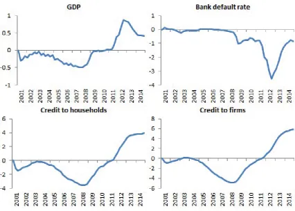
Using these implicit shocks we can simulate the evolution of a slightly altered
version of the model where the parameter for the capital ratio is set at its
opti-mal level. Graph 5 shows the effect, given the observed shocks, of changing this
parameter. They are expressed in percentage level differences of the counterfactual
simulated variables with respect to their observed evolution.
These results show that a higher capital ratio (15.6% instead of 13.2%) would
have had a cost in terms of output and credit levels during the expansion. Yet, it
would have been very effective at reducing the default rate of banks during the crisis,
which in turn would have had a positive impact on credit and GDP: The total size
of the crisis in terms of output, from peak to through, would have been reduced by
2.3
Comparison to alternative welfare measures
To get a broader perspective on the performance of our welfare measure, we
com-pare it to a set of alternative measures outlined in section 2.1.3. Figure 6 shows the
relative performance of our measure against alternatives. The first important thing Figure 4: Shock decomposition
to note is that our welfare criterion outperforms alternative (simplistic) measures
since the gain in welfare from this policy is more balanced compared to the
alter-natives. For example, if one would to use GDP level as the underlying criterion for
optimal capital level setting, then GDP, investment, and housing investment would
be slightly higher compared to the level using our criterion, while credit would be
significantly lower, and average default almost 20% higher. Also, optimal capital
level would be 1% lower compared to the level found here. Alternatively, using the
default rate as the objective criterion, the default rate would indeed be almost 10%
lower compared to the level in this paper, but investment, housing investment, and
com-Figure 5: Difference in variables between the optimal and observed scenario
effects on the rest of the economy. For the remaining criteria (consumption and
number of crises), we find a similar pattern. In that sense, the criterion used here is
much more balanced and (in relative terms) produces less economic costs compared
to alternative criteria.
The other comparison we wish to make is with respect to the consumption
equiv-alence measure of Clerc et al (2015). The graph furthest below on the left in Figure
6 compares the relative gains in welfare of using the stated welfare criterion in
each column compared to ΔW used in the Clerc et al (2015) paper.6 First of all,
pared to what we find here. This is because for the model to further reduce average
default rate compared to the optimal setting in this paper, the optimal capital level
for Euro Area needs to be 2.4% higher (or at 18%), which has highly contractionary
Ɖ Ɖ Ƌ Ő Ɖ /ŶǀĞƐƚŵĞŶƚ;йͿ ƌĞĚŝƚ;йͿ ,ŽƵƐŝŶŐ/ŶǀĞƐƚŵĞŶƚ;йͿ ǀĞƌĂŐĞĚĞĨĂƵůƚ;йͿ tĞůĨĂƌĞ KƉƚŝŵĂůĐĂƉŝƚĂů 'W;йͿ Ϭ͘Ϭϵϱ Ϭ͘ϭ Ϭ͘ϭϬϱ Ϭ͘ϭϭ Ϭ͘ϭϭϱ Ϭ͘ϭϮ Ϭ͘ϭϮϱ Ϭ͘ϭϯ
tĞůĨĂƌĞ 'W ŽŶƐƵŵƉƚŝŽŶ EƵŵďĞƌŽĨ ĐƌŝƐŝƐ ĞĨĂƵůƚƌĂƚĞ ϭϬ͘Ϭ ϭϭ͘Ϭ ϭϮ͘Ϭ ϭϯ͘Ϭ ϭϰ͘Ϭ ϭϱ͘Ϭ ϭϲ͘Ϭ ϭϳ͘Ϭ ϭϴ͘Ϭ
tĞůĨĂƌĞ 'W ŽŶƐƵŵƉƚŝŽŶ EƵŵďĞƌŽĨ ĐƌŝƐŝƐ ĞĨĂƵůƚƌĂƚĞ ͲϬ͘Ϭϰ ͲϬ͘Ϭϯ ͲϬ͘ϬϮ ͲϬ͘Ϭϭ Ϭ Ϭ͘Ϭϭ Ϭ͘ϬϮ Ϭ͘Ϭϯ Ϭ͘Ϭϰ Ϭ͘Ϭϱ Ϭ͘Ϭϲ
tĞůĨĂƌĞ 'W ŽŶƐƵŵƉƚŝŽŶ EƵŵďĞƌŽĨ ĐƌŝƐŝƐ ĞĨĂƵůƚƌĂƚĞ ͲϬ͘ϲ ͲϬ͘ϱ ͲϬ͘ϰ ͲϬ͘ϯ ͲϬ͘Ϯ ͲϬ͘ϭ Ϭ
tĞůĨĂƌĞ 'W ŽŶƐƵŵƉƚŝŽŶ EƵŵďĞƌŽĨ ĐƌŝƐŝƐ ĞĨĂƵůƚƌĂƚĞ ͲϬ͘ϭ ͲϬ͘Ϭϱ Ϭ Ϭ͘Ϭϱ Ϭ͘ϭ Ϭ͘ϭϱ Ϭ͘Ϯ
tĞůĨĂƌĞ 'W ŽŶƐƵŵƉƚŝŽŶ EƵŵďĞƌŽĨ ĐƌŝƐŝƐ ĞĨĂƵůƚƌĂƚĞ ͲϵϬ ͲϴϬ ͲϳϬ ͲϲϬ ͲϱϬ ͲϰϬ ͲϯϬ ͲϮϬ ͲϭϬ Ϭ
tĞůĨĂƌĞ 'W ŽŶƐƵŵƉƚŝŽŶ EƵŵďĞƌŽĨ ĐƌŝƐŝƐ ĞĨĂƵůƚƌĂƚĞ Ϭ Ϭ͘ϭ Ϭ͘Ϯ Ϭ͘ϯ Ϭ͘ϰ Ϭ͘ϱ Ϭ͘ϲ Ϭ͘ϳ Ϭ͘ϴ Ϭ͘ϵ
tĞůĨĂƌĞ 'W ŽŶƐƵŵƉƚŝŽŶ EƵŵďĞƌŽĨ ĐƌŝƐŝƐ
ĞĨĂƵůƚƌĂƚĞ
Figure 6: Long-run impacts on different variables using alternative welfare criteria
it is clear that all the welfare measures outperform the consumption equivalence
measure. Second, the relative gains from using the welfare measure of this paper,
together with consumption and number of crisis criterion, are highest compared to
other alternatives such as GDP and default rate. Finally, note that if the policy
maker wishes to use a simpler (easy to communicate) criterion, he would be as good
off using the aggregate (balanced) consumption or number of crises criterion since
the relative welfare gains compared to the consumption equivalence criterion are the
same, and the macro-financial impacts are very close.
The reasons for the apparent outperformance of the welfare measure in this paper
(and other alternatives) to the consumption equivalence lies in the limitations of the
ΔW measure outlined in section 2.1.3. In particular, since the Clerc et al (2015)
measure puts a higher weight on the welfare of borrowers, it does not fully take into
account the trade-offs between the welfare function of borrowers and savers as one
increases the capital ratio.
3
Optimal Countercyclical Capital Buffers
The capital requirements ratio discussed in the previous section is a static
macropru-dential measure. We now turn to its dynamic counterpart: a rule for countercyclical
buffers. Remember that, according to Basel III and the model set-up,
countercycli-cal buffer is added on top of the static capital requirements, not substituting for
it.
In the area of monetary policy, the Talyor rule has become a standard approach
to model monetary reaction functions and a large literature has studied the general
equilibrium implications of having such a rule, to which variables the optimal rule
should respond to, the optimal coefficients, etc. In the context of macroprudential
policy, the literature on optimal CCyB is much thinner, and we are far away from a
consensus on whether all CCyB rules should have the same features, not to mention
if there may even exist an equivalent to the ‘golden rule’. Said that, we do believe
that discussions and analytics relating to optimal monetary policy may be highly
useful for our purposes not least because, just as a monetary policy rules, it is
time-varying and responds distinctively across the cycle. Likewise, the optimal
rule should balance the benefits of curbing the (financial) cycle without imposing
excessive costs, and thus improving agents’ total welfare. Moreover, there are good
reasons for wanting to openly communicate a rule such that the public can anticipate
the reaction of the central bank and anchor its expectations, just as in the case of
monetary policy. The main difference, however is that CCyB will react to variables
essential to financial stability, which have distinct data-generating process to their
macroeconomic counterparts in a monetary policy rule.7
3.1
Optimality and loss function
CCyB, unlike (optimal) capital requirements, is an instrument affecting the
short-run as it curbs the cycle. In other words, it only affects the dynamics around the
steady state, not the steady state itself. Because of this, agents only care about
the variation in their utility function arguments, where a higher (lower) variation
decreases (increases) their welfare. Hence, they aim to minimise losses that are
generated from variance in these variables. The optimal policy should therefore be
the one that minimizes those losses. But unlike optimal capital requirements, CCyB
rules can react to many variables and there is no obvious outrighta priori candidate.
8Note that we are deriving a welfare optimality criterion for a quasi-linear model that is not log-linearized. By quasi-linear we imply that the model is non-linear in nature, since the default threshold gives rise to at least two states of nature, but that the jump or transition between them is smoothened via use of near-linear numerical methods. Moreover, the model includes a welfare-transfer policy that impacts the income losses and distribution absent any other policy. So, for instance, if there is a bank default, tax policy will be triggered, with subsequent welfare effects without any action on the part of the Central Bank. Considering this, the welfare criterion that is derived will assist us in finding the conditional global optimum. That is different from the unconditional optimal we find for standard linear DSGE models where there are no ex ante policy effects. Hence, the optimum that will be derived with the variance-only loss function, albeit model-consistent, micro-founded, and information efficient, may be different from optima derived using any other version of a welfare function. Nevertheless, for our CCyB purposes here, the second Thus, our objective in this section is two-fold. First, to discover which rule produces
the smallest loss amongst viable alternatives that involve the most relevant financial
stability variables. Second, to determine the weights on each variable in the rule
that generates the least loss. Both aims rely on having defined a clear and easily
quantifiable loss function that is used as objective criterion in the experiments. This
loss function will only contain variance terms of the variables that are fundamental
to consumers’ aggregate utility. As for optimal monetary policy, we obtain this
loss function using the joint utility of all consumers in the model, and derive these
fundamental variance terms using the model’s first principles.8
moment-based loss function is the correct information criterion to be used in finding the optima. 3.1.1 Deriving the second-order loss function
We take the second order approximation to aggregate utility of consumers to derive
our CCyB policy objective function. Since the two households are the only
con-sumers in our setting, the policy objective function will be a weighted average of
the (approximate) utility function of saver-and borrower households, or:
E0
∞
i=0
βt+i[ζUts+ (1−ζ)Utm] (31)
whereζ is the weight of the utility of savers in the policy objective. The two utility
functions are:
E0
∞
i=0 βts+i
logcst+1+νsloghst+i−1− ϕ s
1 +η(l s t+i)1+η
(32)
for savers, while for borrowers it is:
E0
∞
i=0 βtm+i
logcmt+1+νmloghmt+i−1− ϕ m
1 +η(l m t+i)1+η
(33)
We follow the methods proposed by Woodford (2003), Gali and Monacelli (2004),
Chadha et al (2010), and DeFiore and Tristani (2013) to approximate their utility
functions. In words of Woodford (2003), our aims of this exercise are to derive an
explicit expression for the stabilization loss with which we can evaluate alternative
macroprudential policies, and identify those policies that make this quantity as small
as possible. This method is more convenient than other proposed in the literature,
such as the optimal simple policy rule of Levine (1991) in that it is time consistent,
and hence the choice of optimal rule will not depend on the initial level of the policy
stance. Moreover, the loss function is fully model consistent since it is derived from
the model’s micro structure and it captures the total social (consumer) welfare in
the model (unlike the welfare criterion of Schmitt-Grohe and Uribe, 2004).
After derivations in Appendix II, we find that the above expression can be
ap-proximated and re-written using purely quadratic additive terms:
E0
∞
i=0
βt+i(Ut−U) =−1 2E0Σ
∞
i=0βt+iLt+t.i.p+O3 (34)
with Lt=χkσk2+χlsσl2s +χlmσ2lm+χhsσ2hs +χhmσh2m
where χk ≡Y Assα(kss)α−1+ 1, χls ≡((1−α)lsss)−α− 1+ϕsη +1+2η, χlm ≡((1−α)lssm)−α−1+ϕmη + 1+2η, χhs ≡1 +ζνhsh,
and χhm ≡1 + (1−ζ)νhmh.
Using the calibrated values for the Euro Area explained in the 3D model, and
extracting the steady state values for the endogenous variables, we find the following
optimal weights for each of the arguments in the loss function:
χk≡ 5,677∗1∗0.3∗(40,176)−0.7 + 1 = 1,128 (35)
χls ≡((1−0,3)∗1,296)−0,3∗ −1∗(1,296)(1+1)1 + 1
2 = 1,357 (36)
χlm ≡((1−0,3)1,521)−0,3−1∗(1,521)(1+1)1 + 1
2 = 2,006 (37)
χhs ≡1 + 0,475∗ 0,204
40,786 ∗40,786 = 1,097 (38)
χhm ≡1 + (1−0,475)∗ 0,512
Normalizing to 1 for χlm, the respective weights become:
χk≡ 1,128
2,006 = 0,562 (40)
χls ≡ 1,357
2,006 = 0,676 (41)
χlm ≡ 2,006
2,006 = 1 (42)
χhs ≡ 1,097
2,006 = 0,546 (43)
χhm ≡ 1,346
2,006 = 0,670 (44)
3.2
Quantitative results
3.2.1 Optimal CCyB rule
We will now try to find the optimal response rule of regulatory capital buffers to
variables such as credit, housing prices and loan spreads, in order to minimize the
losses generated by excessive volatility in the key model variables (described in the
loss function above). We first do so while keeping the capital ratio at its calibrated
value; the next section, on optimal instrument interaction, will check whether the
optimal CCyB rule changes once the capital ratio has already shifted towards its
optimum value.
It would not be feasible to try all possible functional forms for such a rule, but
we will try at least the most obvious options. We will use the social loss function
defined above both to find the optimal reaction parameters for each specification,
and also to compare different rules once they all use their optimal parameters. As
before, we conduct experiments within a calibration of the model for the Euro Area.
Our two proposed functional forms for the CCyB rule are:
crt=φcrcrfx+φabt+φbqHt (45)
crt =φcrcrfx+φabt+φbRHt (46)
where φcr is total capital requirement at time t, crfx is the fixed (non-cyclical)
component of the capital level, and φa and φb are the parameters that control the
responses of the CCyB rule to the first (a) and second (b) arguments. All terms are
where φcr is total capital requirement at time t, crfx is the fixed (non-cyclical)
component of the capital level, and φa and φb are the parameters that control the
responses of the CCyB rule to the first (a) and second (b) arguments. All terms are
expressed in deviations (gaps) from their steady state values. For each specification
we estimate the optimal value of parameters φa and φb (the responsiveness of total
capital requirement to each argument in the rule) by looking for the values that
minimize the social utility-based loss, as defined above. bt is total credit given by
banks, qtH is the housing price, and RtH the mortgage lending spread.
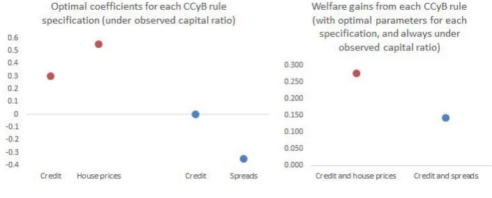
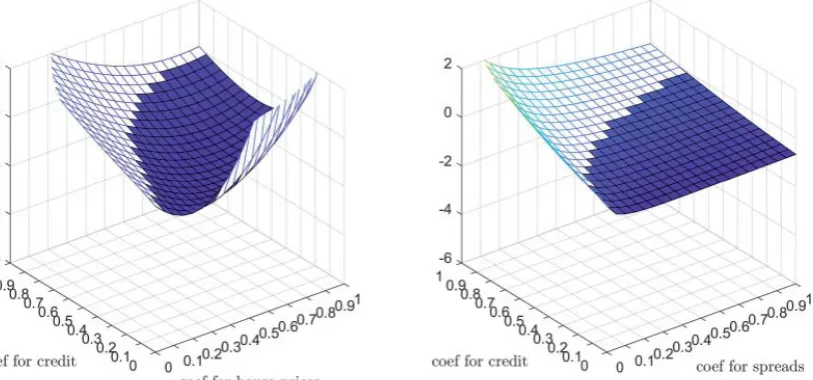
The graphs below show optimal coefficients for each rule when the capital ratio
is at its observed value, and the welfare gains (the reduction in the loss function)
achieved by these rules.
From the Figure 7, out of the specifications that we tested, the preferred rule is
the one that responds to total credit and house prices, and it does so with weights
of approximately 0.3 and 0.6 respectively. The rule that responds to total credit
and credit spreads should not respond to total credit.
These results say that an optimal rule based on credit and house prices would
tend to have balanced positive coefficients for both arguments, whereas a
specifi-cation based on credit and spreads should concentrate on responding to the latter.
An important result coming out of this graph is that, unlike the case of the capital
ratio where there was a very wide range of values that improved welfare compared Figure 7: Optimal CCyB rules and coefficients
To further investigate this issue, the following graphs depict, for each functional
form, the welfare gains obtained for different ranges of values of the parameters φa
andφb. The shaded area represents points where the rule achieves a positive welfare
gain with respect to having an inactive CCyB policy rule. Figure 8 depicts the loss
functions.
to the observed level, in the case of CCyB the range of values achieving welfare
Figure 8: Surface of the loss function for different rules and parameter values
In both graphs, if we setφb = 0 and only allow the CCyB to respond to credit, we
find that the optimal value ofφb is also zero. This implies that CCyB rules can be a
tricky policy instrument. If we consider that the policymaker has uncertainty over
the model underlying the real-world economy (including its weights/coefficients)
and ends up choosing a rule with mispecified (or ”wrong”) coefficients, it seems
uncomfortably likely that this choice will result in a reduction of welfare. This could
also be translated to the case of implementing one-size-fits-all policy across different
economies, which, particularly in Europe, is an issue that should be investigated
further.
4
Optimal instrument interaction
Identifying the optimal instruments in isolation can only be welfare improving within
the reach of each instrument. However, as authorities are activating multiple
macro-prudential instruments, the desire to know their joint impact becomes higher. In
this model, this is relatively straightforward as the two instruments are complements
and are added on top of the other. Although operationally it is relatively simple
to activate both instruments, their joint impact is not easy to pin-down
analyti-cally. In particular, since both instruments tackle financial stability and have an
impact on the financial cycle, it is a priori not clear whether their effects are
com-plementary, substituting, multiplicative, or even counteracting. Moreover, it is not
apparent whether the optimal policy design may change once both instruments are
triggered. To answer these questions, we would need to activate both instruments
while running the model and test two things. First, whether the joint impact from
both optimal instruments is equal to the sum of the two effects individually.
Sec-ond, to check whether there is another combination of policies (in particular another
CCyB rule) that may generate better results. This second experiment would allow
us to understand whether the individual optima remain optimal even under more
complex policy environments. To run these experiments, we use the loss function
defined earlier as our objective criterion to determine the optimal combination since
the instruments are additive and the level of welfare cannot be improved once the
basic (fixed) optimal requirement has been implemented. Thus we add the CCyB
rule on top of the optimal capital requirement to examine the joint effects on losses.9
4.1
Optimal combination of capital-based instruments
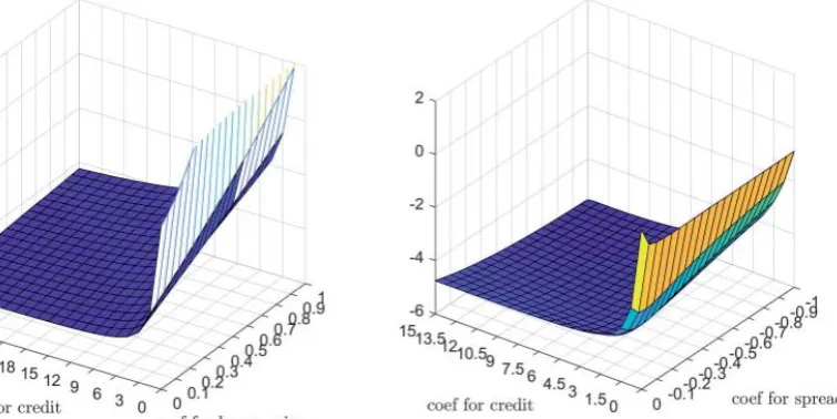
Graphs 9 and 10 repeat the analysis of the previous section, but in a situation in
which the capital ratio is already at its optimal level. With the same functional
forms for the possible CCyB rules, the optimal rule now changes, including the
optimal coefficients.
Figure 9: Optimal CCyB rules and their coefficients under alternative capital re-quirement scenarios
9Note that there is no need to re-optimise capital requirements since the structure and shocks in the model have not changed under this scenario. Moreover, there is no other policy that is activated which may condition the results. Thus, the optimal capital level is unconditional and cross-cutting across both situations. The only policy that may change is the CCyB as it’s additive. Moreover, the new level of welfare (or decrease in losses) is much higher compared
to the case of only one optimal instrument, or the sum of the effects from individual
optimal instruments. Moreover, with a higher capital ratio already in place, the
The graphs that plot the loss function for each pair of parameters now illustrate
a much bigger area of potential improvement:
This suggests that achieving a right balance in terms of the optimal capital ratio
requirements (the policy instrument that affects both levels and variance of the
main macro and financial variables) recognizes more space for the CCyB rule (the
instrument that only affects the variance) to be able to achieve, in a robust manner,
its own goals of reducing excessive volatility in the economy.
Figure 10: Surface of the loss function under optimal capital requirements
4.2
Counterfactuals
As we did in a previous section, we now use the historical shocks retrieved by
the model to simulate, with an alternative calibration (that now includes both the
optimal capital ratio and the associated optimal CCyB rule), to simulate what would
have been the evolution of the economy during the recent boom and crisis if both
instruments had been set optimally in 2001. As we can see in graph 11, adding the
optimal CCyB rule intensifies the effects that we already saw when evaluating the
effects of the optimal capital ratio, but it doesn’t do this in a uniform way: the
bank default rate can’t be improved much farther from what the optimal capital
ratio was already achieving, but on top of that the CCyB rule is still effective in
further reducing the size of GDP and credit fluctuations (providing a higher level
of these variables during the crisis, at the cost of a smaller positive deviation at the
end of the boom).
To further illustrate the effects of these policies, graph 12 depicts the same results
in a different way: the green lines show the observed evolution of the economy (in
counterfactual scenario with both optimal capital and optimal CCyB rule. Here we
see more clearly that the financial cycle is strongly damped by these instruments,
with credit deviating less from its steady state both in good and bad times, and bank
default rate never even approaching the levels that it reached during the second part
Figure 11: Difference in the evolution fo the variables under various scenarios
of the crisis (the reduction in the steady state level of the bank default rate achieved
by the increase in the capital ratio explains the fact that the red dotted line can
be always below zero: it is above its own steady state, but never reaches the levels
from the original one).
The effect in terms of the real cycle (in this case, GDP) is somewhat smaller:
GDP grows less during the boom and falls by less in the second half of the crisis, but
the difference between the observed path and the counterfactual one is admittedly
not as pronounced as in the case of credit or the default rate.
4.3
Impulse response functions
The main channel that explains the improved performance of the economy under
optimal capital ratio and CCyB rules is the way it reacts to financial shocks. Graph
13 shows the IRF of the model to a bank risk shock in three different calibrations:
its optimal value (red dashed line) and one in which, on top of that, the optimal
CCyB rule has also been implemented (blue dashed line).
Figure 12: Evolution of the various variables under realized and optimal joint in-strument scenario
Figure 13: Impulse responses under various scenarios of optimal instruments
0 10 20 30 40 -0.18
-0.16 -0.14 -0.12 -0.1 -0.08 -0.06 -0.04 -0.02
0 GDP
0 10 20 30 40 0
0.1 0.2 0.3 0.4 0.5 0.6 0.7 0.8
Average Bank Default
Baseline CR CR+CCyB
10 20 30 40
-0.35 -0.3 -0.25 -0.2 -0.15 -0.1 -0.05