R E S E A R C H A R T I C L E
Open Access
A random effects meta-analysis model
with Box-Cox transformation
Yusuke Yamaguchi
1*†, Kazushi Maruo
2, Christopher Partlett
3†and Richard D. Riley
4†Abstract
Background: In a random effects meta-analysis model, true treatment effects for each study are routinely assumed to follow a normal distribution. However, normality is a restrictive assumption and the misspecification of the random effects distribution may result in a misleading estimate of overall mean for the treatment effect, an inappropriate quantification of heterogeneity across studies and a wrongly symmetric prediction interval.
Methods: We focus on problems caused by an inappropriate normality assumption of the random effects
distribution, and propose a novel random effects meta-analysis model where a Box-Cox transformation is applied to the observed treatment effect estimates. The proposed model aims to normalise an overall distribution of observed treatment effect estimates, which is sum of the within-study sampling distributions and the random effects
distribution. When sampling distributions are approximately normal, non-normality in the overall distribution will be mainly due to the random effects distribution, especially when the between-study variation is large relative to the within-study variation. The Box-Cox transformation addresses this flexibly according to the observed departure from normality. We use a Bayesian approach for estimating parameters in the proposed model, and suggest summarising the meta-analysis results by an overall median, an interquartile range and a prediction interval. The model can be applied for any kind of variables once the treatment effect estimate is defined from the variable.
Results: A simulation study suggested that when the overall distribution of treatment effect estimates are skewed,
the overall mean and conventionalI2from the normal random effects model could be inappropriate summaries, and
the proposed model helped reduce this issue. We illustrated the proposed model using two examples, which revealed some important differences on summary results, heterogeneity measures and prediction intervals from the normal random effects model.
Conclusions: The random effects meta-analysis with the Box-Cox transformation may be an important tool for examining robustness of traditional meta-analysis results against skewness on the observed treatment effect estimates. Further critical evaluation of the method is needed.
Keywords: Meta-analysis, Random effects model, Skewed data, Box-Cox transformation
Background
Meta-analysis is a useful statistical tool for combining results from independent studies, for example where esti-mates of a treatment effect (e.g odds ratio, mean differ-ence or standardised mean differdiffer-ence) from randomised controlled trials are pooled in order to make infer-ences about an overall summary effect. A random effects
*Correspondence: [email protected] †Equal contributors
1Japan-Asia Data Science, Development, Astellas Pharma Inc., 2-5-1,
Nihonbashi-Honcho, Chuo-ku, 103-8411 Tokyo, Japan Full list of author information is available at the end of the article
meta-analysis model that assumes different true treatment effects underlying different studies is often needed as it allows for unexplained heterogeneity across studies [1]. In the random effects model, the true treatment effects for each study are usually assumed to follow a normal distri-bution; thus, an overall mean (summary) effect is obtained by estimating the mean parameter of this distribution.
In this article, we focus on problems caused by an inap-propriate normality assumption of the random effects distribution, in particular in regard to the impact on the mean effect estimate, quantification of heterogeneity and prediction interval. Turner et al. [2] suggested that
the misspecification of the random effects distribution seriously affected the estimates of the random effects vari-ances. Lee and Thompson [3] showed that the shape of the predictive distributions of the treatment effect was sub-stantially affected by the shape of the assumed random effects distribution. The normality assumption may there-fore be a restrictive assumption for meta-analysts who are interested in producing a summary treatment effect, quantifying heterogeneity and deriving a prediction inter-val, especially if the true random effects distribution is skewed.
Alternative parametric distributions have been consid-ered for the random effects distribution in mixed mod-els; for example, t-distribution [4], gamma or mirrored gamma distribution [2], Laplace (double-exponential) dis-tribution [5], skewed normal or skewed t-disdis-tribution [3], mixture distributions [6]. And also, as an approach to out-liers in meta-analysis, Baker and Jackson [7] proposed a model that allows the random effects to be long-tailed, which provides a down-weighting of outliers and removes the necessity for an arbitrary decision to exclude the out-liers. Gumedze and Jackson [8] used likelihood ratio test statistics to detect and down-weight outliers in the meta-analysis. However, each has disadvantages as discussed in Lee and Thompson [3]; for example, the mixture dis-tributions can fail in situations where there are a few outliers. When assuming a skewed distribution for the random effects in a meta-analysis, the mean and the vari-ance are not appropriate representatives for summarising the skewed true treatment effects. The overall mean for the skewed treatment effects would be pulled in the direc-tion of the extreme observed estimates; hence, it could result in misleading conclusions from the meta-analysis. It is also not straightforward to quantify the impact of het-erogeneity, such as I2, if there is a non-normal random effects distribution. Indeed, Higgins et al. [9] mentioned that some alternative parametric distributions may not have parameters that naturally describe an overall effect, or the heterogeneity across studies.
Here, we propose a novel random effects meta-analysis model, where a Box-Cox transformation [10] is applied to the observed treatment effect estimates. The aim of the Box-Cox transformation is to achieve approximate normality of the overall distribution of the observed treat-ment effect estimates after transformation. The use of the Box-Cox transformation in linear models has been studied extensively [11–14]. In particular, Gurka et al. [15] provided an extension of the Box-Cox transformation to linear mixed models and demonstrated that a sin-gle transformation parameter would simultaneously help achieve normality of both the random effects and the residual error. However, the Box-Cox transformation has not been used commonly in the context of meta-analysis. Indeed, a work by Kim et al. [16] is the only meta-analytic
application of the Box-Cox transformation that we are aware of. They proposed a multivariate response Box-Cox regression model for modelling individual patient data (IPD). However, the approach by Kim et al. [16] cannot apply to the cases of more readily available aggregate data (such as observed estimates of the treatment effect and their standard errors), because their model just allows the individual patient responses to be transformed and thus requires IPD. We rather consider transforming the observed treatment effect estimates using the Box-Cox transformation and suggest summarising the overall effect by an overall median rather than the overall mean, and quantifying the impact of heterogeneity by an interquar-tile range rather than commonly usedI2. The method no longer requires the IPD.
In this section, we introduce two motivating examples which will be used for illustrating the proposed model. In the “Methods” section, we introduce the standard nor-mal random effects models, and describe how to make the Bayesian inference in the random effects meta-analysis from the following viewpoints: the overall mean effect, the heterogeneity and the prediction interval. And then, we describe our new random effects model with the Box-Cox transformation. In the “Results” section, we conduct a simulation study to examine the performance of our pro-posed model under some situations where true random effects follow non-normal distributions, and compare the results with those from the standard normal random effects model. Moreover, we illustrate our proposed model using the examples. Finally, we conclude this article with some discussion.
Motivating examples
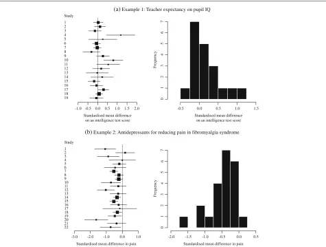
Example 1: Teacher expectancy on pupil IQ
1 2 3 4 5 6 7 8 9 10 11 12 13 14 15 16 17 18 19 Study
0 . 2 0
. 1
- -0.5 0.0 0.5 1.0 1.5
Standardised mean difference on an intelligence test score
-0.5 0.0 0.5 1.0 1.5
Frequency
01234567
Standardised mean difference on an intelligence test score (a) Example 1: Teacher expectancy on pupil IQ
-3.0 -2.0 -1.0 0.0 1.0
1 2 3 4 5 6 7 8 9 10 11 12 13 14 15 16 17 18 19 Study
20 21 22
Standardised mean difference in pain
5 . 0 0 . 0 5
. 1 -0 . 2
- -1.0 -0.5
Standardised mean difference in pain
Frequency
01234567
(b) Example 2: Antidepressants for reducing pain in fibromyalgia syndrome
Fig. 1Forest plot and histogram.a19 experiments investigating teacher expectancy on pupil IQ,b22 studies investigating antidepressants for reducing pain in fibromyalgia syndrome
participants) in the studies, it does suggest the presence of positive skewness in the observed distribution of the estimates.
Example 2: Antidepressants for reducing pain in fibromyalgia syndrome
Hauser et al. [20] reported a meta-analysis of randomised controlled trials to investigate the efficacy of antidepres-sants for fibromyalgia syndrome, which is a chronic pain disorder associated with multiple debilitating symptoms. 22 trials using different classes of antidepressants were involved in the analysis, and estimates of the standard-ised mean difference in pain (for the antidepressant group minus the control group) were combined using a random effects model. The data was obtained from Figure 3 in Riley et al. [21]. Figure 1b shows a forest plot and a simple histogram of estimates of the standardised mean differ-ences, with negative values indicating a benefit for the antidepressants. The histogram suggests the presence of negative skewness on the estimates.
Methods
Normal random effects model
We first consider the standard normal random effects model for a meta-analysis ofk studies. Letyi andσi2be an estimate of a treatment effect and its variance observed from theith study (i = 1,. . .,k), respectively. Then the normal random effects model is given by
yi=θi+i, (1)
θi=θ +ui,
i∼N0,σi2, ui∼N0,τ2
where the within-study varianceσi2is commonly consid-ered to be known. Of key interest is an estimate of the mean parameter of the random effects distribution,θ, as this provides the mean treatment effect of the included studies. Also of interest is an estimate ofτ2, to quantify the amount of heterogeneity and to derive a 95 percent prediction interval [9].
Bayesian estimation of model parameters
We here use a Bayesian approach for estimating param-eters involved in the normal random effects model (1). Marginalising the true treatment effect (θi) from a joint distribution of yi and θi, we have yi ∼ N
θ,τ2+σi2. Given θ andτ2, the conditional density function ofy = (y1,. . .,yk)is written as
p(y|θ,τ2)= k
i=1
1 √
2πτ2+σ2
i
1/2exp
− (yi−θ)2 2τ2+σ2
i
.
Then a posterior distribution ofθandτ2can be given as
pθ,τ2|y∝py|θ,τ2pθ,τ2
wherep(θ,τ2)is a prior density forθ andτ2. Since min-imally informative prior distributions are appropriate in the absence of definite priori information, we here use the following vague priors:
θ ∼ N(0, 10000), (2)
τ ∼ U(0,b)
wherebis a constant value given by practitioners. It is well known that the results from Bayesian meta-analyses could be potentially sensitive to the choice of prior distributions, especially to the prior of the between-study variance τ2 (e.g. see Lambert et al. [22] for the details). Various non-informative priors forτ2have been suggested in previous researches; for example, a uniform prior onτ [23, 24], a uniform prior on log(τ2)[25], an inverse-gamma prior on τ2[26] and a half-Cauchy prior onτ[24]. We consider the uniform prior onτ in the range of(0,b), where the upper limit, b, should be decided according to the individual situations. The uniform prior on the standard deviation increasingly becomes known as a reasonable alternative to a more general inverse-gamma prior on variance (e.g. see Gelman [24] for the details). In practice the sensitivity of specified priors should be investigated by applying many other priors for the parameters or by using prior distribu-tion based on empirical evidence [27, 28], though we in this article avoid the extensive discussion for the prior. In the Bayesian framework, a posterior mean and a 95 per-cent credible interval are commonly used for summarising the posterior distribution. We implement our Bayesian analysis by using Markov chain Monte Carlo (MCMC)
methods, with a free R software and its rstan package (see the Stan Modelling Language User’s Guide and Reference Manual [29] for the details). The source code for conduct-ing meta-analyses with the normal random effects model (1) is shown in Additional file 1.
Quantification of heterogeneity
The magnitude of heterogeneity across studies can be quantified by the posterior estimate of the between-study varianceτ2or its square root. In the Bayesian framework, we obtain the posterior distribution ofτ2and its credible interval, which can be used for quantifying the magnitude of the between-study heterogeneity of the true treatment effects. However, the between-study variance may be sen-sitive to the metric of the treatment effect, and thus this is not necessarily appropriate for the purpose of comparing several meta-analyses in terms of the heterogeneity [30]. If we are interested in what proportion of the observed vari-ance reflects real differences in the treatment effect, theI2 proposed by Higgins and Thompson [30] is useful for this purpose. Under the normal random effects model (1), the I2is expressed as a function ofτ2, given by
I2= τ
2
τ2+s2 (3)
where
s2= (k−1)
k i=11/σi2
k i=11/σi2
2
−k
i=1
1/σi22
. (4)
Here,s2is referred to as ‘typical’ within-study variance. In this article, we calculateI2based on the estimatedτ2 dur-ing each sample of the Bayesian estimation process; that is, we summarise the posterior distribution ofI2derived by using samples ofτ2drawn from its posterior distribution.
Prediction interval
In the Bayesian framework, a predictive distribution of the treatment effect in a new study is given by
p(θnew|y)=
pθnew|θ,τ2
pθ,τ2|ydθdτ2. (5)
limits. When interest lies in predicting probability that the treatment is effective by more than a clinically important difference in a new study, we can find this by calculat-ing the proportion of samples drawn from the predictive distribution which satisfy a specified criteria for the effec-tiveness of the treatment (e.g. odds ratio<80 percent). The sampling can be achieved by first drawing samples of parameters from the posterior distributionpθ,τ2|y and then drawing samples frompθnew|θ,τ2
with fixed parameters obtained in the previous step [4]. In the sec-ond step, the drawing is performed byθnew∼Nθ,τ2. In this manner, the prediction interval accounts for the het-erogeneity in true treatment effects and naturally incorpo-rates all parameter uncertainty (e.g. inθandτ2). It should be interpreted differently from the credible interval for the mean effect, which only indicates the uncertainty in the mean effect itself, not the entire distribution of true treatment effects across studies [21].
Random effects model with Box-Cox transformation Box-Cox transformation
Before giving our proposed model, we first introduce the Box-Cox transformation for a standard consideration of a continuous variable. The aim of the Box-Cox transfor-mation is to achieve approximate normality of a variable (say,yi) after transformation [10]. Roughly saying, it can be used for changing scale of data so that the trans-formed data are distributed symmetrically. In particular, we consider a normalised shift transformation given by
yi(λ,α)=
⎧ ⎪ ⎨ ⎪ ⎩
(yi+α)λ−1
λg(α)˙ λ−1 , λ=0 log(yi+α)g˙(α), λ=0
(6)
foryi+α >0 (i=1,. . .,k), where we keepyifor ease of notation, thoughyicould refer to any continuous measure (not just an effect size).λandαdenote a transformation and a shift parameter respectively, and these parameters are estimated from the observed data.g˙(α)is a geomet-ric mean of yi + α for i = 1,. . .,k. The normalisation using the geometric meang˙(α)could lead a stable estima-tion ofλandα, in comparison with a standard Box-Cox transformation without the normalisation.
To be exact, it is proper to assume that the transformed variableyi(λ,α) follows a truncated normal distribution except for the case of λ = 0, because of the condi-tion thatyi+α must be a positive value. When interest lies in inference in original scale before transformation (not in the scale after transformation), we need to specify the distribution of the observed values before the Box-Cox transformation and deal with the truncation precisely [31–34]. However, these are beyond the scope of this article. For mathematical convenience, we below assume
that the transformed variable yi(λ,α) follows a normal distribution with no consideration of the truncation.
Proposed meta-analysis model and its estimation
Let yi’s be the treatment effect estimates (e.g. log odds ratio or mean difference) from the available studies in a meta-analysis. We propose the following random effects model for the Box-Cox transformedyi:
yi(λ,α) = μi+i, (7) μi = μ+ui,
i∼N0,φ2i(λ,α), ui∼N(0,τ2).
The model structure is basically same as the normal ran-dom effects model (1), though now the Box-Cox trans-formation (6) is applied to the observed treatment effect estimates for each study andμi denotes a true effect of the Box-Cox transformed variable yi(λ,α) which has a ‘known’ variance ofφ2i(λ,α)(see section below). The pro-posed model aims to improve the overall normality of the observed treatment effects estimates (yi) across stud-ies; their overall distribution is the sum of the random effects distribution of true effects and the within-study sampling distribution of estimates. As long as the stud-ies have reasonable sample size, the within-study sampling distribution ofyiwill be approximately normal due to the central limit theorem. However, there is no such guaran-tee for the random effects distribution [7], and thus any asymmetry in the random effects distribution will conse-quently cause asymmetry in the overall distribution for yi. The following processes are required to implement the proposed random effects model (7).
Definition of variance of the Box-Cox transformed treatment effect estimate In the proposed model (7), the variance of the Box-Cox transformed treatment effect estimate, φi2(λ,α); i.e. the variance of yi(λ,α) givenμi, must be defined. Since the variance needs to be assigned for each study separately, we here approximate the vari-ance ofyi by a first order Taylor series aboutyi(λ,α) = E[yi(λ,α)] as follows:
V[yi]≈V[yi(λ,α)]
∂yi
∂yi(λ,α)
yi(λ,α)=E[yi(λ,α)]
2
= ⎧ ⎪ ⎪ ⎨ ⎪ ⎪ ⎩
V[yi(λ,α)]g˙(α)2λ−2
λg˙(α)λ−1E[y
i(λ,α)]+1
2/λ−2 , λ=0
V[yi(λ,α)]
˙
g(α)2 exp 2E[y
i(λ,α)]
˙
g(α)
, λ=0
.
Box-Cox transformed treatment effect estimate, written by
φ2
i(λ,α)≈
⎧ ⎪ ⎪ ⎪ ⎨ ⎪ ⎪ ⎪ ⎩
σ2
i ˙ g(α)2λ−2
λg(α)˙ λ−1μ+12−2/λ, λ=0
σ2
ig(α)˙ 2exp
− 2μ
˙ g(α)
, λ=0
(8)
where recall α is the shift parameter, λis the transfor-mation parameter,g(α)˙ is the geometric mean ofyi+α fori = 1,. . .,k,μis the mean parameter of the random effects distribution in the transformed scale andσi2is the within-study variance from the ith study. The relation-ship between variances before and after transformation has been applied for stabilising variance [35, 36] or rep-resenting inhomogeneity variances in linear models with Box-Cox transformation weighting [37].
Frequentist estimation ofλand α We treat the trans-formation parameterλand the shift parameterαas non-stochastics; i.e. we first estimate these parameters by a maximum likelihood estimation, and then make inference about the other parametersμandτ2conditioning onλ= ˆ
λandα= ˆα, whereλˆandαˆare maximum likelihood esti-mates ofλandα respectively. Maruo and Goto [34] has investigated the influence of not considering the uncer-tainty associated with estimation of λ, and showed the confidence interval around the median from an univari-ate analysis with the Box-Cox transformation was slightly liberal (from two to three percent).
A log likelihood function for(μ,τ2,λ,α)is given by
l(μ,τ2,λ,α)= k
i=1
− 1
2log
τ2+φ2
i(λ,α)
− (yi(λ,α)−μ)2 2(τ2+φ2
i(λ,α))
.
(9)
A grid search procedure is one simple approach for find-ingλˆ andαˆ which maximises the log likelihood (9) with respect to λ and α. For a large set of values for (λ,α), the log likelihood can be rewritten as l(μ,τ2,λ,α) =
lλ,α(μ,τ2) where μ and τ2 vary but λ and α are fixed. Maximisinglλ,α(μ,τ2)with respect toμandτ2, we obtain their estimates for the fixedλandαas
ˆ
μ(λ,α),τˆ2(λ,α)=arg max μ,τ2
lλ,αμ,τ2.
Substituting the estimates μ(λˆ ,α) and τˆ2(λ,α) into
lλ,α(μ,τ2), then we have a log likelihood lλ,α(μ(λˆ ,α), ˆ
τ2(λ,α))for the fixedλandα. Then, we obtain a set of
(λ,α) for which the log likelihood takes the largest value as the approximate values ofλˆandαˆ.
An issue known as non-regular problem is caused in the maximum likelihood estimation of α because the range of the distribution is determined by the unknown shift parameter α [38, 39]. For example, it is argued that the likelihood function of α fails to have a local maximum [38]. In this article, we focus on the inference in the orig-inal scale before transformation; hence, we assume the concern about the estimation of α would not have sub-stantial impact than if we were interested in the exact estimation of the transformation and the shift parameter (λ and α) themselves. This could be an area of further research.
Bayesian estimation of model parameters Givenλˆand ˆ
α (i.e. optimum transformation of the treatment effect, yi(λˆ,α)ˆ fori = 1,. . .,k and their variances), we take a Bayesian approach to estimation of the unknown param-eters from the Box-Cox meta-analysis model (7), μand τ2. Marginalising the true treatment effect (μi) from a joint distribution of yi(λˆ,α)ˆ andμi, we haveyi(λˆ,α)ˆ ∼ N(μ,τ2+φi2(λˆ,α))ˆ . The posterior distribution ofμand τ2is given by
p(μ,τ2|y;λˆ,α)ˆ ∝p(y|μ,τ2;λˆ,α)ˆ p(μ,τ2)
where
p(y|μ,τ2;λˆ,α)ˆ = k
i=1
1 √
2π(τ2+φ2
i(λˆ,α))ˆ 1/2
exp
− (yi(λˆ,α)ˆ −μ)2 2(τ2+φ2
i(λˆ,α))ˆ
. (10)
We assume the vague priors for μ and τ2 in the same way as (2); i.e. μ ∼ N(0, 10000) and τ ∼ U(0,b), where b is a constant value given by practitioners. It is straightforward to draw samples from the posterior dis-tribution (10) by MCMC. The source code for conducting meta-analyses with the proposed model (7) is shown in Additional file 1, which includes the step of finding the maximum likelihood estimates ofλandα.
Interpretation of results
A median overall treatment effect We first define a true effect of the untransformed variableyias
θi∗≡
⎧ ⎨ ⎩
λg(α)˙ λ−1μi+11/λ−α, λ=0
exp μi
˙
g(α)
−α, λ=0 (11)
distribu-tion ofθi∗, not ofμi), it is useful to consider statistical measures induced from the distribution ofθi∗. Note that μi ∼ N(μ,τ2), then thepth percentile of the distribu-tion ofμi is given byμ+τzp, wherezp denotes thepth percentile of a standard normal distribution. Thus, substi-tutingμ+τzpinto (11), we obtain thepth percentile of the distribution ofθi∗as
ξp=
⎧ ⎨ ⎩
λg(α)˙ λ−1(μ+τzp)+11/λ−α, λ=0
expμ+τzp
˙
g(α)
−α, λ=0 . (12)
And also, the median of the distribution ofθi∗is given by
ξ50= ⎧ ⎨ ⎩
λg(α)˙ λ−1μ+11/λ−α, λ=0
exp˙g(α)μ −α, λ=0 . (13)
The median (13) can now be used for the inference of an overall (summary) treatment effect on the original scale. We recommend using the median as a representative of centre of skewed distributions, which is more robust than the mean against the skewness and the outliers on the observed treatment effect estimates.
Quantification of heterogeneity using the ratio of IQR squares Under the normal random effects model (1), the between-study variance τ2 and the I2 can be used for quantifying the magnitude and the impact of the het-erogeneity across studies, respectively. However, when considering skewed distributions, variance is not the most appropriate measure for describing the spread of the distributions. In general, the variance is defined as an expected value of the squared deviation from the mean, though in the skewed-data situation the data is no longer distributed symmetrically around the mean. Due to the skewness or the heavy-tailedness of the data, the variance may lead a wrongly large spread of the distribution. That is, under the proposed model (7), the variance of the dis-tribution ofθi∗does not provide appropriate information about the heterogeneity across studies. For this reason, we here use an interquartile range (IQR) instead of the vari-ance, which is defined as the difference between 75th and 25th quantiles for the distribution ofθi∗; i.e.ξ75−ξ25from (12). Against the skewness of the data, the IQR is known as a more robust measure of spread than the variance. Note that the IQR of a normal distribution is exactly equal to the product of its standard deviation andz75−z25. There-fore, if we observe normally distributed treatment effect estimates, a measure of
ξ75−ξ25
z75−z25
(14)
from the proposed model (7) would be close to the square root of between-study variance from the normal random
effects model (1). For this comparability, we recommend using the measure of (14), which is known as normalised IQR, for quantifying the magnitude of the heterogeneity.
We also define a criteria for quantifying the impact of the heterogeneity for the skewed treatment effects. Note that yi(λ,α) ∼ Nμ,τ2+φ2i(λ,α), then the pth per-centile of the distribution ofyi(λ,α)is given byμ+(τ2+ φ2
i(λ,α))1/2zp. Substituting a ‘typical’ within-study vari-ance like (4) into theφi2(λ,α)and back-transforming the pth percentile into the original scale, we obtain thepth percentile of the distribution ofyias
νp=
⎧ ⎪ ⎪ ⎨ ⎪ ⎪ ⎩
λg(α)˙ λ−1(μ+(τ2+d2)1/2zp)+11/λ−α, λ=0
exp
μ+(τ2+d2)1/2z
p ˙
g(α)
−α, λ=0
(15)
where
d2= (k−1)
k
i=11/φ2i(λ,α)
k
i=11/φ2i(λ,α)
2
−k
i=1
1/φi2(λ,α)2
denotes the ‘typical’ within-study variance of the Box-Cox transformed variables. Obviously from the definition by (3), theI2has an aspect of the proportion of the between-study variation that is due to the heterogeneity across studies (variance ofθi∗) to the total variation in the treat-ment effect estimates (total variance ofyi). In the similar concept, we now consider using a ratio of IQR squares alternative to theI2, which is defined as
(IQR of the distribution ofθi∗)2 (IQR of the distribution ofyi)2 =
(ξ75−ξ25)2
(ν75−ν25)2
. (16)
The ratio of IQR squares would be comparable with the I2when the treatment effect estimates are normally dis-tributed, because of the comparability between the IQR and the between-study variance.
Prediction interval Under the proposed model (7), we first consider a predictive distribution of the Box-Cox transformed treatment effect which is given by
p(μnew|y;λ,α)=
p(μnew|μ,τ2)p(μ,τ2|y;λ,α)dμdτ2.
step, the drawing is performed byμnew∼N(μ,τ2). Then, we obtain the samples from the predictive distribution of the treatment effect by back-transforming the samples of μnewas
θnew∗ = ⎧ ⎨ ⎩
λg˙(α)λ−1μnew+1
1/λ−α , λ=0
exp μnew ˙ g(α)
−α, λ=0
. (17)
A (100−q) percent prediction interval can be obtained by taking (q/2)th and (100−q/2)th quantiles of samples drawn from the predictive distribution (17). Again, note that this is just one option for obtaining the 95 percent prediction interval as mentioned in the previous section.
Another transformation for dealing with the negative skewness
As described in the previous section, the Box-Cox trans-formation (6) requires the condition thatyi+αmust be a positive value fori=1,. . .,k, which can cause difficulty in estimating the model parameters. This may also be more problematic when the treatment effect estimates have negative skewness, because the shift parameter is subject to inflation in such situation. In order to avoid the negative skewness on the treatment effect estimates, we here con-sider another transformation using a sign inversion. The transformation with the sign inversion described below will be applied only when the observed treatment effect estimates are negatively skewed.
We first distinguish which direction the skewness is in on the treatment effect estimates. A sample skewness with inverse-variance weightings defined as
k i=1
y
i−¯yw
sw
3
σ2
i
k i=11/σi2
(18)
can be used for this, where
¯ yw=
k
i=1yi/σi2
k
i=11/σi2
, s2w=
k
i=1(yi− ¯yw)2/σi2 k
i=11/σi2 .
If the weighted sample skewness (18) take a negative value, we invert the sign of the treatment effect estimates (i.e. multiply the estimates by −1) and then apply the Box-Cox transformation to the inverted estimates. That is, we use the following transformation for the negatively skewed data:
yi(λ,α)=
(−y
i+α)λ−1
λh(α)˙ λ−1 , λ=0 log(−yi+α)h˙(α), λ=0
(19)
whereh˙(α)is now a geometric mean of−yi+α fori = 1,. . .,k. For each study, the same within-study variances can be assigned to the inverted treatment effect estimates.
The random effects model (7) with the transformation (19) is applied in the same manner as the implement-ing procedures described in the previous section. And also, instead of (11), the true effect of the untransformed variableyiis now defined as
θi∗≡
⎧ ⎪ ⎨ ⎪ ⎩
−λh˙(α)λ−1μi+11/λ+α, λ=0 −exp μi
˙
h(α)
+α, λ=0
.
Then, instead of (12) and (15), we have thepth percentiles of the distribution ofθi∗andyias follows:
ξp= ⎧ ⎪ ⎨ ⎪ ⎩
−λh˙(α)λ−1(μ+τzp)+1
1/λ
+α, λ=0
−exp
μ+τz
p
˙
h(α)
+α, λ=0
and νp= ⎧ ⎪ ⎪ ⎪ ⎨ ⎪ ⎪ ⎪ ⎩
−λh˙(α)λ−1(μ+(τ2+d2)1/2zp)+1
1/λ
+α, λ=0
−exp
μ+(τ2+d2)1/2z
p ˙
h(α)
+α, λ=0
which can be used for estimating the overall median effect and the ratio of IQR squares. The prediction interval is also obtained by the same procedure described in the pre-vious section, except for the step of back-transforming the samples ofμnew. Instead of (17), we here use
θ∗ new= ⎧ ⎪ ⎨ ⎪ ⎩
−λh(α)˙ λ−1μ new+1
1/λ
+α, λ=0
−exp μnew ˙ h(α)
+α, λ=0
for obtaining samples from the predictive distribution.
Implementation of our proposed model
We here summarise an implementation procedure of our proposed model using the Box-Cox transformation with the sign inversion for negatively skewed data:
1. Calculate the weighted sample skewness (18). 2. If the weighted sample skewness calculated in Step 1
takes a negative value, invert the sign of observed treatment effect estimates and then move to Step 3; otherwise just move to Step 3.
3. Calculate the maximum likelihood estimates of the transformation (λ) and the shift (α) parameter using the log-likelihood function (9).
4. Perform the Bayesian estimation (MCMC sampling) for the other parameters given the maximum likelihood estimates of the transformation and the shift parameter.
6. Draw samples from the predictive distribution using the MCMC samples obtained in Step 4, and calculate the prediction interval.
Steps 1 and 2 are needed only when applying the sign inversion. Without the sign inversion, we will begin the procedure from Step 3.
Results
Simulation study
We conducted a simulation study to examine the compar-ative performance of the standard normal random effects model (1) and the proposed model (7). Since the proposed model allows the presence of skewness on the treatment effect estimates, we supposed some situations where the true treatment effects had a skewed distribution, and compared results from the two models in terms of the estimation of overall effect and the quantification of het-erogeneity. We also supposed another situation where the treatment effect estimates were normally distributed. In such situation, the two models are expected to provide similar results.
Design
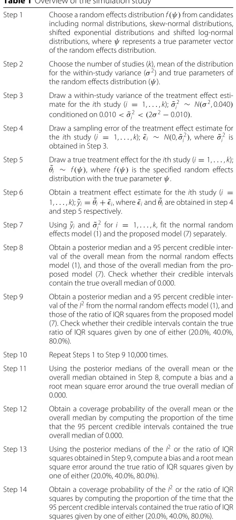
Table 1 shows an overview of the simulation study. Under several scenarios of random effects distributions, we con-sidered simulating 10,000 meta-analyses of k studies, where the number of studies was fixed in each simulation withk∈ {5, 10, 20, 40}. A treatment effect estimateyiand a within-study varianceσi2for theith study (i=1,. . .,k) were randomly generated with the procedures of Steps 1-6 in Table 1. We below describe each step in detail.
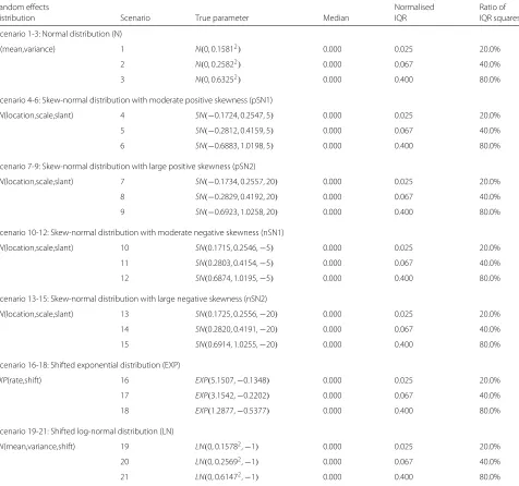
In Step 1, a random effects distribution was chosen from candidates. We considered a variety of random effects distributions (normal distribution, skew-normal distribu-tion [40, 41], shifted exponential distribudistribu-tion and shifted log-normal distribution) which a true treatment effectθi for theith study was drawn from. The normal distribu-tions were chosen for examining how the proposed model worked in the case of symmetrically distributed data that could be precisely fit by the normal random effects model. The skew-normal distributions were chosen for imitating situations with moderate to large skewness in a positive and a negative directions. The shifted exponential and the shifted log-normal distributions were chosen for imi-tating situation with heavy-tailed data as well as positive skewness. True parameters in the random effects distribu-tions were specified so that the median of the distribution became equal to zero, and the normalised IQR square of the distribution became one of either (0.025, 0.067, 0.400). The setting of zero overall median means a null hypothesis of no treatment effect. The scenario of the true normalised IQR square is equivalent to setting the true ratio of the IQR squares as (20.0%, 40.0%, 80.0%) which are obtained
Table 1Overview of the simulation study
Step 1 Choose a random effects distributionf(ψ)from candidates including normal distributions, skew-normal distributions, shifted exponential distributions and shifted log-normal distributions, whereψrepresents a true parameter vector of the random effects distribution.
Step 2 Choose the number of studies (k), mean of the distribution for the within-study variance (σ2) and true parameters of the random effects distribution (ψ).
Step 3 Draw a within-study variance of the treatment effect esti-mate for theith study (i = 1,. . .,k);σ˜2
i ∼ N(σ2, 0.040) conditioned on 0.010<σ˜2
i < (2σ2−0.010).
Step 4 Draw a sampling error of the treatment effect estimate for theith study (i = 1,. . .,k);˜i ∼ N(0,σ˜i2), whereσ˜i2 is obtained in Step 3.
Step 5 Draw a true treatment effect for theith study (i=1,. . .,k);
˜
θi ∼ f(ψ), wheref(ψ)is the specified random effects distribution with the true parameterψ.
Step 6 Obtain a treatment effect estimate for theith study (i =
1,. . .,k);˜yi= ˜θi+ ˜i, where˜iandθ˜iare obtained in step 4 and step 5 respectively.
Step 7 Using˜yiandσ˜i2fori = 1,. . .,k, fit the normal random effects model (1) and the proposed model (7) separately.
Step 8 Obtain a posterior median and a 95 percent credible inter-val of the overall mean from the normal random effects model (1), and those of the overall median from the pro-posed model (7). Check whether their credible intervals contain the true overall median of 0.000.
Step 9 Obtain a posterior median and a 95 percent credible inter-val of theI2from the normal random effects model (1), and those of the ratio of IQR squares from the proposed model (7). Check whether their credible intervals contain the true ratio of IQR squares given by one of either (20.0%, 40.0%, 80.0%).
Step 10 Repeat Steps 1 to Step 9 10,000 times.
Step 11 Using the posterior medians of the overall mean or the overall median obtained in Step 8, compute a bias and a root mean square error around the true overall median of 0.000.
Step 12 Obtain a coverage probability of the overall mean or the overall median by computing the proportion of the time that the 95 percent credible intervals contained the true overall median of 0.000.
Step 13 Using the posterior medians of theI2or the ratio of IQR squares obtained in Step 9, compute a bias and a root mean square error around the true ratio of IQR squares given by one of either (20.0%, 40.0%, 80.0%).
Step 14 Obtain a coverage probability of theI2or the ratio of IQR squares by computing the proportion of the time that the 95 percent credible intervals contained the true ratio of IQR squares given by one of either (20.0%, 40.0%, 80.0%).
Table 2Scenarios of random effects distributions and their true parameters
Random effects Normalised Ratio of
distribution Scenario True parameter Median IQR IQR squares
Scenario 1-3: Normal distribution (N)
N(mean,variance) 1 N(0, 0.15812) 0.000 0.025 20.0%
2 N(0, 0.25822) 0.000 0.067 40.0%
3 N(0, 0.63252) 0.000 0.400 80.0%
Scenario 4-6: Skew-normal distribution with moderate positive skewness (pSN1)
SN(location,scale,slant) 4 SN(−0.1724, 0.2547, 5) 0.000 0.025 20.0%
5 SN(−0.2812, 0.4159, 5) 0.000 0.067 40.0%
6 SN(−0.6883, 1.0198, 5) 0.000 0.400 80.0%
Scenario 7-9: Skew-normal distribution with large positive skewness (pSN2)
SN(location,scale,slant) 7 SN(−0.1734, 0.2557, 20) 0.000 0.025 20.0%
8 SN(−0.2829, 0.4192, 20) 0.000 0.067 40.0%
9 SN(−0.6923, 1.0258, 20) 0.000 0.400 80.0%
Scenario 10-12: Skew-normal distribution with moderate negative skewness (nSN1)
SN(location,scale,slant) 10 SN(0.1715, 0.2546,−5) 0.000 0.025 20.0%
11 SN(0.2803, 0.4154,−5) 0.000 0.067 40.0%
12 SN(0.6874, 1.0195,−5) 0.000 0.400 80.0%
Scenario 13-15: Skew-normal distribution with large negative skewness (nSN2)
SN(location,scale,slant) 13 SN(0.1725, 0.2556,−20) 0.000 0.025 20.0%
14 SN(0.2820, 0.4191,−20) 0.000 0.067 40.0%
15 SN(0.6914, 1.0255,−20) 0.000 0.400 80.0%
Scenario 16-18: Shifted exponential distribution (EXP)
EXP(rate,shift) 16 EXP(5.1507,−0.1348) 0.000 0.025 20.0%
17 EXP(3.1542,−0.2202) 0.000 0.067 40.0%
18 EXP(1.2877,−0.5377) 0.000 0.400 80.0%
Scenario 19-21: Shifted log-normal distribution (LN)
LN(mean,variance,shift) 19 LN(0, 0.15782,−1) 0.000 0.025 20.0%
20 LN(0, 0.25692,−1) 0.000 0.067 40.0%
21 LN(0, 0.61472,−1) 0.000 0.400 80.0%
Figure S7 show density functions of the random effects distribution for the scenarios 1-3, 4-6, 7-9, 10-12, 13-15, 16-18 and 19-21, respectively.
In Step 2, we set the number of studies, mean of the distribution for the within study variance and true param-eters of the random effects distribution. In Steps 3-6, we obtained treatment effect estimates for each study. In par-ticular, the within-study variance σi2 was drawn from a normal distribution with meanσ2and variance 0.040 con-ditioned on 0.010< σi2< (2σ2−0.010). The mean of the normal distribution, σ2, was chosen so that the ‘typical’ within-study variance (4), which depended on the number of studies involved in the meta-analysis, became 0.100 on average. We set the value ofσ2to either 0.1089, 0.1122,
0.1147, 0.1158 in each simulation withk = 5, 10, 20, 40, respectively.
In Steps 11-14, we calculated the following quantities for comparing the two models (normal random effects model/proposed model):
• Bias around the true overall median: (mean of the posterior medians of the overall mean/the overall median)−(true overall median of 0.000)
• Root mean square error (RMSE) around the true
overall median: ((standard deviation of the posterior medians of the overall mean/the overall
median)2+(bias around the true overall median)2)1/2
• Coverage probability of the true overall median (%): the proportion of the time that the 95 percent credible intervals of the overall mean/the overall median contained the true overall median of 0.000
• Bias around the true ratio of IQR squares: (mean of the posterior medians of theI2/the ratio of IQR squares)−(true ratio of IQR squares given by one of either (20.0%, 40.0%, 80.0%))
• RMSE around the true ratio of IQR squares: ((mean
of the posterior medians of theI2/the ratio of IQR squares)2+(bias around the true ratio of IQR squares)2)1/2
• Coverage probability of the true ratio of IQR squares (%): the proportion of the time that the 95 percent credible intervals of theI2/the ratio of IQR squares contained the true ratio of IQR squares given by one of either (20.0%, 40.0%, 80.0%)
We notice that using the terms of bias, RMSE and cov-erage probability for the results from the normal random effects model is not necessarily correct. This is because the normal random effects model provided the results of overall mean and I2, which were not the targeted true values (or the reference values). However, in this arti-cle, the overall median and the ratio of IQR squares are highly recommended for representing the overall effect and quantifying the heterogeneity in the meta-analysis of skewed data, respectively. Then, the above quantities are useful for assessing how the findings under the two mod-els can be different from the recommended inferential measures in skewed-data situations.
Estimation
Before estimation of model (7) for a particular simulated dataset, the grid search procedure was performed for esti-matingλandα for the dataset. The candidate values of λwere specified in a range of−3.00 ≤ λ ≤ 6.00 with a step size of 0.01. We considered constituting a subset of αas the minimum values of{(yi+α) : i = 1,. . .,k}; i.e. α∗ = α+min{y
i : i= 1,. . .,k}. The candidate values of α∗were specified in a range of 0.01 ≤ α∗ ≤ 2.01 with a
step size of 0.10.
We used the normal and the uniform prior for the mean and the variance parameter respectively, as described in
the previous section. The upper limit of the uniform prior distribution onτ was given byb = 10 for each model. For the Bayesian estimation of model (1) and (7), the iter-ative process of the MCMC algorithm produced three chains each with 20,000 samples of parameters. We dis-carded the first 2,000 samples (so-called burn-in samples) in order to prevent dependence on the starting values. And also, we took a sample at only every 2nd itera-tion (thinning) in order to avoid autocorrelaitera-tion between the samples taken. Therefore in total, 24,000 samples of parameters were drawn. We graphically checked the con-vergence of MCMC sampling using first 5 simulations for each scenario, with no diagnostic methods.
Results
Additional file 2: Table S1, Table S2, Table S3 and Table S4 show results from the two models, for each scenario of the number of studiesk= 5, 10, 20 and 40, respectively. And also, Additional file 2: Table S5 and Table S6 show sum-mary statistics of estimates for the transformation (λ) and the shift (α) parameter, for the scenario of the number of studiesk=40. Note that the summary statistics were cal-culated using 10,000 estimates of the parameters for each scenario of random effects distribution. To make clear the differences between the two models, we depicted the bias, the RMSE and the coverage probability in the following figures:
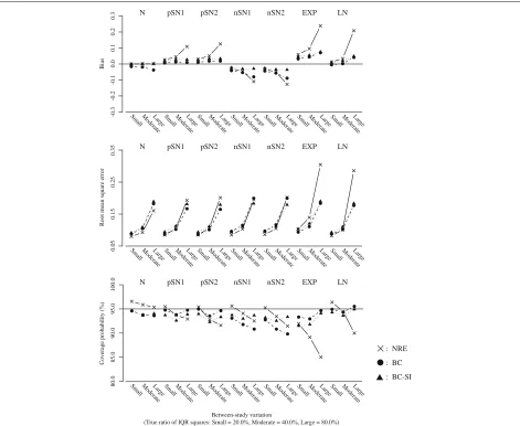
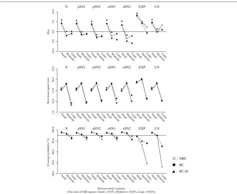
• Figure 2 plots the results for the overall mean or the overall median, with the between-study variation (the true ratio of IQR squares: Small = 20.0%, Moderate= 40.0%, Large=80.0%) on the horizontal axis. The number of studies was fixed ask = 20.
• Figure 3 plots the results for theI2or the ratio of IQR squares, with the between-study variation (the true
ratio of IQR squares: Small=20.0%, Moderate=
40.0%, Large=80.0%) on the horizontal axis. The number of studies was fixed ask = 20.
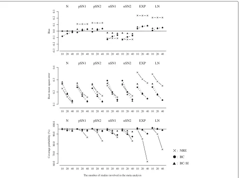
• Figure 4 plots the results for overall mean or the overall median, with the number of studies (k = 10, 20 and 40) on the horizontal axis. The true ratio of IQR squares was fixed as 80.0% (i.e. the scenario of large between-study variation).
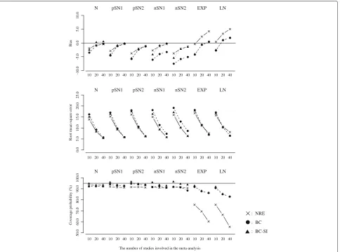
• Figure 5 plots the results for theI2or the ratio of IQR squares, with the number of studies (k = 10, 20 and 40) on the horizontal axis. The true ratio of IQR squares was fixed as 80.0% (i.e. the scenario of large between-study variation).
N pSN1 pSN2 nSN1 EXP LN
-0.3
-0.2
-0.1
0.0
0.1
0.2
0.3
Small
nSN2
ModerateLar
geSmall ModerateLargeSmall ModerateLargeSmall ModerateLargeSmall ModerateLargeSmall ModerateLargeSmall ModerateLarge
Bias
N pSN1 pSN2 nSN1 EXP LN
0.05
0.15
0.25
0.35
Small
nSN2
ModerateLar
geSmall ModerateLargeSmall ModerateLargeSmall ModerateLargeSmall ModerateLargeSmall ModerateLargeSmall ModerateLarge
Root mean square error
N pSN1 pSN2 nSN1 EXP LN
80.0
85.0
90.0
95.0
100.0
Small
nSN2
ModerateLar
geSmall ModerateLargeSmall ModerateLargeSmall ModerateLargeSmall ModerateLargeSmall ModerateLargeSmall ModerateLarge
Coverage probability (
)
Between-study variation
: NRE
: BC
: BC-SI
Fig. 2Bias, RMSE and coverage probability of the overall mean or the overall median for the scenario of the number of studiesk=20. The overall mean from the normal random effects model (cross/solid line), and those of the overall median from the proposed model (black circle/broken line: Box-Cox transformation,black triangle/dotted line: Box-Cox transformation with the sign inversion)
skewness (nSN1), the skew-normal with large negative skewness (nSN2), the shifted exponential (EXP) and the shifted log-normal (LN) from left to right. And also, in each figure, (i) cross marks and solid lines represent the normal random effects model, (ii) black circle marks and broken lines represent the proposed model using Box-Cox transformation (6), (iii) black triangle marks and dotted lines represent the proposed model using Box-Cox trans-formation with the sign inversion (19) for the negatively skewed data. We below refer to the normal random effects model, the proposed model without and with the sign inversion as NRE, BC and BC-SI respectively.
Overall treatment effect When the normal distributions were assumed as the true random effects distribution, the NRE and the BC-SI provided unbiased estimations of the overall effect, regardless of the scenarios of the
between-study variation and the number of studies. The overall median from the BC was subject to a negative bias in the scenario of the large between-study variation and the small number of studies, though this bias decreased as the number of studies increased. The NRE, the BC and the BC-SI provided similar RMSEs, except for the scenario of the small number of studies where the RMSEs from the NRE were smaller than those from the BC and the BC-SI. The coverage probabilities from the NRE were slightly larger than those from the BC and the BC-SI in all the sce-narios, but all these coverage probabilities were close to the nominal level of 95 percent.
N pSN1 pSN2 nSN1 EXP LN
-10.0
-5.0
0.0
5.0
10.0
Small
nSN2
ModerateLar
geSmall ModerateLargeSmall ModerateLargeSmall ModerateLargeSmall ModerateLargeSmall ModerateLargeSmall ModerateLarge
Bias
N pSN1 pSN2 nSN1 EXP LN
5.0
10.0
15.0
20.0
Small
nSN2
ModerateLar
geSmall ModerateLargeSmall ModerateLargeSmall ModerateLargeSmall ModerateLargeSmall ModerateLargeSmall ModerateLarge
Root mean square error
N pSN1 pSN2 nSN1 EXP LN
60.0
7
0.0
80.0
90.0
100.0
Small
nSN2
ModerateLar
geSmall ModerateLargeSmall ModerateLarg e
Small ModerateLar
geSmall ModerateLargeSmall ModerateLargeSmall ModerateLarge
Between-study variation
25.0
: NRE
: BC
: BC-SI
Fig. 3Bias, RMSE and coverage probability of theI2or the ratio of IQR squares for the scenario of the number of studiesk=20. TheI2from the normal random effects model (cross/solid line), and those of the ratio of IQR squares from the proposed model (black circle/broken line: Box-Cox transformation,black triangle/dotted line: Box-Cox transformation with the sign inversion)
variation. In the scenarios of the positive skewness (pSN1 and pSN2), the biases of the overall mean from the NRE increased positively; conversely in the scenarios of neg-ative skewness (nSN1 and nSN2), those increased nega-tively. The degree of bias was larger in the scenario of the large skewness (pSN2 and nSN2). And also, regard-ing the overall means from the NRE in the scenarios of the large between-study variation and the large number of studies, the RMSEs were inflated and the coverage prob-abilities were substantially below the nominal level of 95 percent. On the other hand, the overall medians from the BC and the BC-SI had the smaller biases regardless of the scenarios of the between-study variation and the num-ber of studies. In the scenario of the negative skewness (nSN1 and nSN2) and the large between-study variation, the BC was subject to a negative bias, though this bias decreased as the number of studies increased. The BC
and the BC-SI provided quite similar RMSEs and cover-age probabilities in the scenarios of the positive skewness (pSN1 and pSN2); while, in the scenarios of the negative skewness (nSN1 and nSN2) and the large between-study variation, the coverage probabilities from the BC were below the nominal level of 95 percent. This indicates that the BC could have difficulty in dealing with the negatively skewed data as expected, but the BC-SI performs well.
N pSN1 pSN2 nSN1 EXP LN
-0.3
-0.2
0.0
0.2
0.3
10
nSN2
20 40
Bias
N pSN1 pSN2 nSN1 EXP LN
0.1
0
.2
0.3
nSN2
Root mean square error
N pSN1 pSN2 nSN1 EXP LN
60.0
70.0
80.0
90.0
100.0
nSN2
The number of studies involved in the meta-analysis
0.4
10 20 40 10 20 40 10 20 40 10 20 40 10 20 40 10 20 40
10 20 40 10 20 40 10 20 40 10 20 40 10 20 40 10 20 40 10 20 40
10 20 40 10 20 40 10 20 40 10 20 40 10 20 40 10 20 40 10 20 40
-0.1
0.1
: NRE
: BC
: BC-SI
Fig. 4Bias, RMSE and coverage probability of the overall mean or the overall median for the scenario of true ratio of IQR squares = 80.0% (large between-study variation). The overall mean from the normal random effects model (cross/solid line), and those of the overall median from the proposed model (black circle/broken line: Box-Cox transformation,black triangle/dotted line: Box-Cox transformation with the sign inversion)
be because the scenarios including larger number of stud-ies tended to generate more heavy-tailed data. On the other hand, the overall medians from the BC and the BC-SI were similar and had much smaller biases in com-parison with the overall means from the NRE. The BC and the BC-SI also provided similar results of the RMSE and the coverage probability, which were much better than those from the NRE especially in the scenarios of the large between-study variation and the large number of studies.
In summary, we found that the overall mean from the NRE could be substantially influenced by the skewness on the random effects distribution. Taking into account that the overall mean from the NRE was pulled in the direc-tion of skewness and had the lower coverage probability, the NRE might therefore produce overall effect estimates that do not reflect the median treatment effect if the over-all distribution of treatment effect estimates is skewed or heavy-tailed. Moreover, it was indicated that the sign inversion in the Box-Cox transformation could be an
effective way for precisely estimating the overall median of the negatively skewed treatment effect estimates.
Quantification of heterogeneity When the normal dis-tributions were assumed as the true random effects distri-bution, the NRE, the BC and the BC-SI provided similar results of the bias, the RMSE and the coverage probability, regardless of the scenarios of the between-study variation and the number of studies.
N pSN1 pSN2 nSN1 EXP LN
-10.0
-5.0
0.0
5.0
10.0
10
nSN2
20 40
Bias
N pSN1 pSN2 nSN1 EXP LN
0.0
5.0
10.0
nSN2
Root mean square error
N pSN1 pSN2 nSN1 EXP LN
50.0
70.0
80.0
9
0.0
100.0
nSN2
The number of studies involved in the meta-analysis
15.0
10 20 40 10 20 40 10 20 40 10 20 40 10 20 40 10 20 40
10 20 40 10 20 40 10 20 40 10 20 40 10 20 40 10 20 40 10 20 40
10 20 40 10 20 40 10 20 40 10 20 40 10 20 40 10 20 40 10 20 40
20.0
25.0
60.0
: NRE
: BC
: BC-SI
Fig. 5Bias, RMSE and coverage probability of theI2or the ratio of IQR squares for the scenario of true ratio of IQR squares = 80.0% (large between-study variation). TheI2from the normal random effects model (cross/solid line), and those of the ratio of IQR squares from the proposed model (black circle/broken line: Box-Cox transformation,black triangle/dotted line: Box-Cox transformation with the sign inversion)
indicates that the BC could have difficulty in dealing with the negatively skewed data.
When the shifted exponential and the shifted log-normal distributions were assumed as the true random effects distribution, the I2 values from the NRE were larger than the ratios of IQR squares from the BC and the BC-SI in the scenarios of the large between-study varia-tion. The RMSEs from the NRE, the BC and the BC-SI were quite similar, though the coverage probabilities ofI2 from the NRE were seriously below the nominal level of 95 percent in the scenarios of the large between-study vari-ation, compared with those of the ratios of IQR squares from the BC and the BC-SI. This became more noticeable as the number of studies increased, which would be again because the scenarios including larger number of stud-ies tended to generate more heavy-tailed data. The BC and the BC-SI provided quite similar results of the bias, the RMSE and the coverage probability, regardless of the scenarios of the between-study variation and the number of studies.
In summary, we found that theI2 from the NRE was influenced by the skewness on the random effects dis-tribution. In particular, the heavy-tailed data seriously affected the estimation ofI2in the NRE. Moreover, it was again indicated that the sign inversion in the Box-Cox transformation could be an effective way for precisely esti-mating the ratios of IQR squares of the negatively skewed treatment effect estimates.
probabilities from the BC and the BC-SI were below nom-inal level of 95 percent for almost all the scenarios. In particular, the BC-SI provided around 90 percent cover-age probabilities for the scenarios of the small and the moderate between-study variation. In contract, the cover-age probabilities from the NRE were substantially above the nominal level of 95 percent. These indicate an issue of meta-analysing the small number of studies. In regard to the quantification of heterogeneity, the NRE, the BC and the BC-SI were subject to large positive bias of theI2 or the ratio of IQR squares, which inflated their RMSEs. From these findings, we conclude our proposed model is applicable even when the number of studies is 5, but may have difficulty in ensuring sufficient accuracy in estima-tion of the overall treatment effect and quantificaestima-tion of heterogeneity.
Application
Consider now application to the examples described in the previous section. We applied the normal random effects model (1) and the proposed model (7) to each example, and estimated the posterior distributions of parameters of interest in each model. The transforma-tion with the sign inversion was also applied to example 2 (the weighted sample skewnesses were 2.123 and−1.847 in example 1 and 2 respectively). Note that the trans-formation with the sign inversion is applied only when the observed treatment effect estimates are negatively skewed.
Estimation
Before estimation of model (7) for each example, the grid search procedure was performed for estimatingλandα. The candidate values of λ were specified in a range of −3.00 ≤ λ ≤ 6.00 with a step size of 0.01. We consid-ered constituting a subset ofαas the minimum values of {(yi+α):i=1,. . .,k}; i.e.α∗=α+min{yi:i=1,. . .,k}. The candidate values of α∗ was specified in a range of 0.01≤α∗≤2.01 with a step size of 0.10.
We used the normal and the uniform prior for the mean and the variance parameter respectively, as described in the previous section. The upper limit of the uniform prior distribution on τ was given by b = 10 for each model. For the Bayesian estimation, the iterative process of the MCMC algorithm produced three chains each with 2,000,000 samples of parameters. We discarded the first 5000 samples (so-called burn-in samples) in order to pre-vent dependence on the starting values. And also, we took a sample at only every 5th iteration (thinning) in order to avoid autocorrelation between the samples taken. There-fore in total, 1,185,000 samples of parameters were drawn. We again graphically checked whether the burn-in sam-ples were sufficient and that the MCMC chains converged, with no diagnostic methods.
Overall treatment effect and quantification of heterogeneity Table 3 shows the posterior median and the 95 per-cent credible interval of: the overall mean and the square root of between-study variance from the NRE, the overall median and the normalised IQR from the BC and the BC-SI. In example 1, the posterior median of the overall mean from the NRE was noticeably larger than that of the overall median from the BC. In example 2, the posterior medi-ans of the overall mean from the BC and the BC-SI were quite similar to each other, but noticeably larger than that of the overall mean from the NRE. Note that the observed treatment effect estimates in example 1 were subject to the positive skewness, in contrast we observed the nega-tively skewed treatment effect estimates in example 2; this causes the overall means from NRE to be forced toward the direction of skewness in each example.
In both examples, the 95 percent credible intervals of the overall median from the BC and the BC-SI were sub-stantially narrower than those of the overall mean from the NRE, indicating the misspecification of the random effects distribution led to the inflation of the between-study variance in the NRE. Indeed, in both examples, we found larger posterior medians of the square root of between-study variance from the NRE in comparison with the normalised IQRs from the BC and the BC-SI. Figure 6a shows the posterior distributions of the overall mean from the NRE and those of the overall median from the BC and the BC-SI for each example. The overall medians had sharper peak of posterior densities than the overall mean in both examples.
Table 4 shows the posterior medians and the 95 per-cent credible intervals of the I2 from the NRE, and the ratio of IQR squares from the BC and the BC-SI. In exam-ple 2, the results from the BC and the BC-SI were quite similar. The ratios of IQR squares from the BC and the BC-SI were substantially smaller than the I2’s from the NRE in both examples. The NRE would conclude moder-ate heterogeneity for the meta-analyses of the examples; however, taking into account the inflation of the between-study variance from the NRE, theI2’s are more likely to be overestimated. On the other hand, the BC and the BC-SI would conclude low heterogeneity for the same examples.
Prediction interval and predictive probability
Table 3Posterior median and 95 percent credible interval of: overall mean and square root of between-study variance from the normal random effects model, overall median and normalised IQR from the proposed model
NRE BC BC-SI
Square root of
between-study Normalised Normalised
Overall mean variance Overall median IQRa Overall median IQRa
Post. (s.d.) Post. (s.d.) Post. (s.d.) Post. (s.d.) Post. (s.d.) Post. (s.d.)
(95% CI) (95% CI) (95% CI) (95% CI) (95% CI) (95% CI)
Example 1: Teacher expectancy on pupil IQ
0.083 (0.061) 0.146 (0.087) 0.030 (0.051) 0.084 (0.074) n/a n/a
(−0.021,0.222) (0.011,0.344) (−0.058,0.144) (0.004,0.278)
Example 2: Antidepressants for reducing pain in fibromyalgia syndrome
−0.418 (0.067) 0.164 (0.097) −0.369 (0.056) 0.094 (0.077) −0.361 (0.057) 0.098 (0.081)
(−0.567,−0.298) (0.013,0.384) (−0.489,−0.267) (0.005,0.291) (−0.484,−0.259) (0.005,0.306)
aNormalised IQR=(ξ
75−ξ25)/(z75−z25)
Post.: posterior median, s.d.: standard deviation, CI: credible interval
NRE: normal random effects model, BC: proposed model using Box-Cox transformation
BC-SI: proposed model using Box-Cox transformation with the sign inversion for negatively skewed data
the predictive distributions from the NRE, the BC and the BC-SI for each example. The 95 percent prediction inter-vals were also depicted on the same panel, where the cross, the black circle and the black triangle represent the medi-ans of predictive distribution from the NRE, the BC and
the SI, respectively. We found the BC and the BC-SI provided skewed prediction intervals, which reflects the asymmetry detected and the asymmetric predictive distribution; whereas the NRE method gave symmetrical prediction intervals in both examples.
(a) Posterior distribution of overall mean
and overall median
(b) Predictive distribution with
Example 1
-0.6 -0.4 -0.2 0.0 0.2 0.4 0.6 0.8
02468
Density
Standardised mean difference on an intelligence test score
Example 2
02468
Density
-1.2 -1.0 -0.8 -0.6 -0.4 -0.2 0.0 0.2
Standardised mean difference in pain
-0.6 -0.4 -0.2 0.0 0.2 0.4 0.6 0.8
02468
Density
Standardised mean difference on an intelligence test score
02468
Density
-1.2 -1.0 -0.8 -0.6 -0.4 -0.2 0.0 0.2
Standardised mean difference in pain
10 10
Fig. 6Posterior and predictive distribution.aPosterior distribution of the overall mean from the normal random effects model (solid line), and of the overall median from the proposed model (broken line: Box-Cox transformation,dotted line: Box-Cox transformation with the sign inversion),b