doi:10.3926/jiem.2008.v1n2.p4-15 ©© JIEM, 2008 – 01(02): 4-15 - ISSN: 2013-0953
Variations in the efficiency of a mathematical programming
solver according to the order of the constraints in the model
Rafael Pastor
Universitat Politècnica de Catalunya (SPAIN)
[email protected]
Received September 2008
Accepted November 2008
Abstract:
It is well-known that the efficiency of mixed integer linear mathematical
programming depends on the model (formulation) used. With the same mathematical
programming solver, a given problem can be solved in a brief calculation time using one
model but requires a long calculation time using another. In this paper a new, unexpected
feature to be taken into account is presented: the order of the constraints in the model can
change the calculation time of the solver considerably. For a test problem, the Response
Time Variability Problem (RTVP), it is shown that the ILOG CPLEX 9.0 optimizer
returns a ratio of 17.47 between the maximum and the minimum calculations time
necessary to solve optimally 20 instances of the RTVP, according to the order of the
constraints in the model. It is shown that the efficiency of the mixed integer linear
mathematical programming depends not only on the model (formulation) used, but also
on how the information is introduced into the solver.
Keywords: mixed integer linear mathematical programming, response time variability
problem, combinatorial optimization
1 Introduction
doi:10.3926/jiem.2008.v1n2.p4-15 ©© JIEM, 2008 – 01(02): 4-15 - ISSN: 2013-0953
motorcycle assembly line and in Pastor et al. 2008 it was applied to solve the case of a woodturning company). The technique is well-known and reliable but it must be handled carefully. It is known that its efficiency depends on the model (formulation) used: with the same mathematical programming solver, a given problem can be solved in a brief calculation time using one model but requires a long calculation time using another. Therefore, as stated by Billionnet (1999, p. 105): “Given a problem with a few dozen of variables one cannot be confident that integer programming will work until it has been tried on realistic instances”.
Several techniques have been used to improve the efficiency of this tool. A standard technique is the elimination of symmetries: Margot (2007), for example, presents techniques for handling symmetries in integer linear programs in which variables can take integer values, which extends previous research that dealt exclusively with binary variables. Tightening the definition of the data and introducing redundant constraints have also provided good results: Corominas et al. (2006), for example, demonstrated the importance of modelling, as well as the huge impact that redundant constraints and the elimination of symmetries have on the effectiveness of MILPs for solving the Response Time Variability Problem (RTVP), an NP-hard scheduling problem (Corominas et al., 2007); the total computation time taken to solve 20 instances dropped from 38,603 to 398 seconds and its practical limit to obtaining optimal solutions was increased from 25 to around 40 units to be scheduled.
This paper argues that the order of the constraints in a model can have a considerable effect on the time that a mathematical programming solver takes to solve a problem optimally. Lets us, for example, take three sets of constraints (A, B and C) of a problem to be solved. To introduce the sets of constraints in the mathematical programming solver in the order A-B-C, A-C-B, B-A-C, B-C-A, C-A-B and C-B-A is not indifferent and can cause its efficiency to vary considerably. This new, unexpected feature that must be taken into account in mathematical programming has not been presented previously (to the best of the authors’ knowledge).
doi:10.3926/jiem.2008.v1n2.p4-15 ©© JIEM, 2008 – 01(02): 4-15 - ISSN: 2013-0953
sets of constraints the solver takes only 335 seconds, whereas with another one it takes 5,851 seconds. It is shown that the efficiency of the mixed integer linear mathematical programming depends not only on the model (formulation) used, but also on how the information is introduced into the solver.
The rest of the paper is organized as follows. Section 2 presents the RTVP. Section 3 describes the computational experiment carried out. Finally, Section 4 is devoted to the conclusions.
2 The test problem: the Response Time Variability Problem
The Response Time Variability Problem (RTVP) occurs whenever products, clients or jobs need to be sequenced so as to minimize variability in the time between the instants at which they receive the necessary resources. It was recently defined in the literature and first presented by Corominas et al. (2007), who proved that it is NP-hard.
This problem has a broad range of real-world applications. For example, it can be used in the automobile industry to sequence the models to be produced on a mixed-model assembly line (Monden, 1983). Other contexts in which the RTVP appears are the computer multi-threaded systems and network servers (Waldspurger and Weihl, 1995), the periodic machine maintenance problem (Bar-Noy et al., 2002), the scheduling of advertising slots for television (Brusco, 2008), the design of sales catalogs (problem introduced in Bollapragada et al., 2004) and the scheduling of waste collection (Herrmann, 2007).
The abovementioned applications are examples of a very common situation in which a resource must be used successively by different units and it is important to schedule them in such a way that the different types of units share the resource in some fair manner. The RTVP proposes a measure of fairness: to minimize the variability of the distance (measured, for example, in number of slot times) between any two consecutive units of the same product (event, job or client); i.e., to have the distances between any two given consecutive units of the same product as constant as possible.
The RTVP is formulated as follows. Let be the number of products, the
doi:10.3926/jiem.2008.v1n2.p4-15 ©© JIEM, 2008 – 01(02): 4-15 - ISSN: 2013-0953
. Let be a solution of an instance in the RTVP that consists of a
circular sequence of units , where is the unit sequenced in
position of sequence . For all products in which , let be the distance
between the positions at which the units and of product are found (i.e.
the number of positions between the units, where the distance between two consecutive positions is considered equal to 1). As the sequence is circular, position
1 comes immediately after position ; therefore, is the distance between the
first unit of product in a cycle and the last unit of the same product in the
preceding cycle. Let be the average distance between two consecutive units of
product . For all products in which , is equal to . The
objective is to minimize the .
For example, let , , and ; thus, , , and
Any sequence is a feasible solution. For example, the sequence (C, A, C, B,
C, B, A, C) is a solution, where
.
doi:10.3926/jiem.2008.v1n2.p4-15 ©© JIEM, 2008 – 01(02): 4-15 - ISSN: 2013-0953
considered. The model to be tested, which is presented in the Annex, consists of an objective function to be minimised, labelled (1), and 10 sets of constraints, labelled (2) to (11).
3 Computational experiment
Using the RTVP as the test problem, a computational experiment was performed in order to show that the order of the constraints in the model can have a considerable effect on the calculation time of the mathematical programming solver. The basic data used for the experiment are as follows:
• The 20 instances in Computational Experiment 1 in Corominas et al. (2006)
were used. In short, was between 21 and 40 units, was between 3
and 12 products, and was between 1 and 15 units.
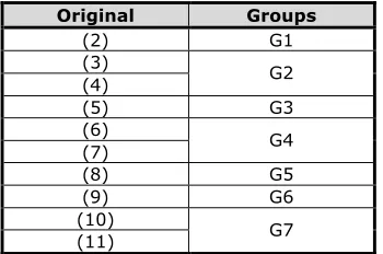
• Sets (2) to (11), the 10 sets of constraints of the model shown in the
Annex, were grouped into seven groups of constraints (G1 to G7). All possible permutations of these seven groups of constraints were carried out; therefore, 7! MILP models were generated and solved optimally (5,040
models). Table 1 shows the 10 original sets of constraints and
the seven groups of constraints that were used to test the order .
The grouping of the original sets of constraints was carried out in accordance with the similarity between the characteristics of the RTVP that were modeled by the restrictions. As explained later in this paper, grouping the constraints into seven groups shows that the order of the constraints in the model has a decisive influence on the efficiency; therefore, it was not necessary to generate and solve optimally the 10! MILP models (it would indeed be highly time-consuming: solving the 7! MILP models took 4,550,156 seconds).
• The MILP models were solved to optimality using the ILOG CPLEX 9.0
doi:10.3926/jiem.2008.v1n2.p4-15 ©© JIEM, 2008 – 01(02): 4-15 - ISSN: 2013-0953
Original Groups
(2) G1
(3)
(4) G2
(5) G3
(6)
(7) G4
(8) G5
(9) G6
(10)
(11) G7
Table 1. “Grouping of the original sets of constraints”.
The 5,040 MILP models were generated and solved optimally for each of the 20 test instances (a total of 100,800 models). Obviously, the number of variables and constraints of the 5,040 models were the same for each instance, because the only difference between these MILP models was the order of the seven groups of constraints. For each of the 5,040 models the sum of the calculation time of the 20 instances was obtained. Table 2 shows the permutations required by the minimum and maximum calculation times (in seconds).
Permutation of the groups Time (in seconds)
G5_G2_G3_G6_G1_G7_G4 335
G6_G5_G4_G2_G7_G3_G1 5.851
Table 2. “Best and worst permutations of the groups of constraints”.
Table 2 shows the ILOG CPLEX 9.0 optimizer takes only 335 seconds for
permutation G5_G2_G3_G6_G1_G7_G4, whereas for permutation
G6_G5_G4_G2_G7_G3_G1 it takes 5,851 seconds. That is, in order to solve 20 instances of this test problem, the order of the constraints in the model returns a ratio of 17.47 between the maximum and the minimum calculation times of the ILOG CPLEX solver.
4 Conclusions
doi:10.3926/jiem.2008.v1n2.p4-15 ©© JIEM, 2008 – 01(02): 4-15 - ISSN: 2013-0953
In order to reveal this difference in performance, a computational experiment was conducted in which the Response Time Variability Problem (RTVP) was solved using the ILOG CPLEX 9.0 optimizer. It returned a ratio of 17.47 between the maximum and the minimum calculation times necessary to solve optimally 20 instances of the RTVP, according to the order of the constraints in the model. With one permutation of the sets of constraints the solver needs only 335 seconds, whereas with another one it needs 5,851 seconds. It has thus been shown that the efficiency of the mixed integer linear mathematical programming depends not only on the model used, but also on how the information is introduced into the solver.
Because the ILOG CPLEX 9.0 optimizer is commercial software, it is very difficult for the authors to explain its performance. One hypothesis, which is not confirmed, is that the order in which the variables are handled in the search process depends on the order of the constraints in the model. Obviously, if we formalize the RTVP with another model (or we solve another problem) the difference in performance according to the order of the constraints in the model could be lower, but it could also be even higher.
Future research work will involve checking if this new, unexpected feature is also showed when another mathematical programming solver is used. The possibility to establish a formalised procedure to achieve, a priori, the best order of the constraints in the model is another area of future research.
Annex
The RTVP model to be tested is specifically as follows.
Data:
Number of products
Total number of units
Number of units of product to be scheduled ;
doi:10.3926/jiem.2008.v1n2.p4-15 ©© JIEM, 2008 – 01(02): 4-15 - ISSN: 2013-0953
Average distance between two consecutive units of product :
Set of products with :
Lower and upper bound on the distance between two consecutive units
of product
First and last position that can be occupied by unit of product
Set of positions that can be occupied by unit of product :
Variables:
Position of unit of product
1 if and only if unit of product is placed in position (
)
1 if and only if the distance between units and of product is
greater than or equal to
Model:
(1)
(2)
doi:10.3926/jiem.2008.v1n2.p4-15 ©© JIEM, 2008 – 01(02): 4-15 - ISSN: 2013-0953
(4)
(5)
(6)
(7)
(8)
(9)
(10)
(11)
Objective function (1) minimises the response time variability. (2) provides the
position of unit of product . (3) and (4) ensure that the distance between
units and of product is equal to an integer value between and . (4)
refers to the distance between the first unit of product in a cycle and the last unit of the same product in the preceding cycle. (5) imposes the consistency of values
for . (6) ensures that one and only one unit is placed in each position of the
doi:10.3926/jiem.2008.v1n2.p4-15 ©© JIEM, 2008 – 01(02): 4-15 - ISSN: 2013-0953
product with the largest is fixed in the first position of the sequence (we can
assume, without loss of generality, that this product is product 1); then (8) calculates two values for the sequence, considering it first in clockwise order and then in anticlockwise order and it is imposed that the value for the former is less than or equal to the value for the latter. With (9) a value is calculated for the
sequence by shifting the units of product with the largest (we can assume,
without loss of generality, that this product is product 1); then, it is imposed that the value of the first sequence is less than or equal to the “value” of the other
sequences. Finally, for each product , it is imposed, over variables , that
the sum of the distances between its units is equal to ((10) and (11)).
Acknowledgments
The author is very grateful to Professor Albert Corominas (Technical University of Catalonia) for his valuable comments, which have helped to enhance this paper. This research has been supported by the Spanish MCyT project DPI2007-61905 co-financed by the FEDER
References
Bar-Noy, A., Bhatia, R., Naor, J., & Schieber, B. (2002). Minimizing service and
operation costs of periodic scheduling. Mathematics of Operations Research, 27,
518-544.
Billionnet, A. (1999). Integer programming to schedule a hierarchical workforce with variable demands. European Journal of Operational Research, 114, 105–114.
Bollapragada, S., Bussieck, M.R., Mallik, S. (2004). Scheduling commercial videotapes in broadcast television. Operations Research, 52(5), 679-689.
Brusco, M.J. (2008). Scheduling advertising slots for television. Journal of the
Operational Research Society, 59, 1363-1372.
doi:10.3926/jiem.2008.v1n2.p4-15 ©© JIEM, 2008 – 01(02): 4-15 - ISSN: 2013-0953
Corominas, A., Pasto,r R., & Plans, J. (2008). Balancing assembly line with skilled and unskilled workers. OMEGA The International Journal of Management Sciences, 36, 1126–1132.
Corominas, A., Kubiak, W., & Moreno, N. (2007). Response time variability. Journal of Scheduling, 10, 97–110.
García, A., Pastor, R., & Corominas, A. (2006). Solving the Response Time
Variability Problem by means of metaheuristics. Frontiers in Artificial Intelligence
and Applications, 146, 187–194.
García-Villoria, A., Pastor, R., & Corominas, A. (2007). Solving the Response Time
Variability Problem by means of the Cross-Entropy Method. International Journal
of Manufacturing Technology and Management (to be published).
García-Villoria, A., & Pastor, R. (2008ª). Solving the Response Time Variability
Problem by means of the Electromagnetism-like Mechanism. Working paper
IOC-DT-P-2008-03, Universitat Politècnica de Catalunya, Spain (available at http://hdl.handle.net/2117/2013).
García-Villoria, A., & Pastor, R. (2008b). Solving the Response Time Variability
Problem by means of a Psychoclonal Approach. Journal of Heuristics.
doi:10.1007/s10732-008-9082-2.
García-Villoria, A., & Pastor, R. (2009). Introducing dynamic diversity into a
discrete Particle Swarm Optimization. Computers & Operations Research, 36(3),
951-966.
Herrmann, J.W. (2007). Generating Cyclic Fair Sequences using Aggregation and Stride Scheduling. Technical Report, University of Maryland, USA.
Monden, Y. (1983). Toyota Production Systems. Industrial Engineering and
Management Press: Norcross, GA.
Pastor, R., Altimiras, J., & Mateo, M. (2008). Planning production using
mathematical programming: The case of a woodturning company. Computers &
doi:10.3926/jiem.2008.v1n2.p4-15 ©© JIEM, 2008 – 01(02): 4-15 - ISSN: 2013-0953
Margot, F. (2007). Symmetric ILP: Coloring and small integers. Discrete
Optimization, 4, 40–62.
Salkin, H.M., & Mathur, K. 1989. Foundations of integer programming,
North-Holland, Amsterdam.
Waldspurger, C.A., & Weihl, W.E. (1995). Stride scheduling: deterministic
proportional-share resource management. Technical Memorandum MIT/LCS/TM-528. MIT, Laboratory for Computer Science, Cambridge.
©© Journal of Industrial Engineering and Management, 2008 (www.jiem.org)
Article's contents are provided on a Attribution-Non Commercial 3.0 Creative commons license. Readers are allowed to copy, distribute and communicate article's contents, provided the author's and Journal of Industrial Engineering and Management's names are included. It must not be used for commercial purposes. To see the complete