Issues
ISSN: 2146-4138
available at http: www.econjournals.com
International Journal of Economics and Financial Issues, 2019, 9(2), 110-114.
Determinants of Return on Assets and Implications on Stock
Price Changes Level
Yani Riyani*, Kartawati Mardiah, Linda Suherma
Politeknik Negeri Pontianak, Indonesia. *Email: [email protected]
Received: 27 December 2018 Accepted: 28 February 2019 DOI: https://doi.org/10.32479/ijefi.7616
ABSTRACT
This study aims to determine the effect of loan to deposit ratio (LDR) and non-performing loans (NPL) on return on assets (ROA) and Implications for
stock price rate of change using SPSS 16.0 statistical software. In this study, there are 4 variables: LDR and NPL as independent variables (X1 and X2)
and ROA s and Stock Price Rate of Change as a dependent variable (Y) and (Z). The research method used is a causal associative method that aims to determine the relationship between two or more variables. Effect of LDR, NPL to ROAs. Based on the results of SPSS processing, it can be concluded
that the influence of LDR and NPL to levels not significantly change in the stock price. While the level of stock price changes is influenced by the LDR and NPL amounted to 2.10% while the remaining 97.90% is influenced by other factors.
Keywords: Loan to Deposit Ratio, Non Performing Loan, Return on Assets, Stock Price
JEL Classifications: G32, G38, G28
1. INTRODUCTION
The ability of a company to generate profits in its operations is a
major focus on the company’s performance appraisal; because of
the profits the company will be able to known to the company’s ability to fulfill obligations to its investors and also an important
element in the creation of corporate value that shows its prospects
in the future. The level of corporate profitability can be seen from the financial statements that are periodically updated as one of
the obligations to public companies listed on the Indonesia stock
exchange. The financial statements provide raw data onto figures that can be further analyzed.
The level of corporate profitability on fundamental analysis is
usually measured from several aspects, in public companies listed
on the Indonesia Stock Exchange, the financial ratios often used
in analyzing stock price changes are loan to deposit ratio (LDR), non performing loan (NPL) and return on assets (ROA). Then the
value of the financial ratios can be used as the basis of assessment/
eligibility from determining the portfolio policy of investors.
In connection with the above issues, the authors propose a thesis with the subject of the discussion entitled “analysis of the effect of LDR and NPL on ROA and its implication on stock price change rate (case study
at the banks listed in indonesia stock exchange period 2016-2017).”
The purpose of this study is as follows:
a. To know the effect of LDR and NPL simultaneously affect ROA
at banks listed in Indonesia stock exchange period 2016-2017.
b. To know the effect of ROAs to the rate of change of stock price
at banks listed in stock exchange Indonesia period 2016-2017.
c. To know the effect of LDR and NPL jointly affect the rate of change of share price at banks listed in Indonesia stock
exchange period 2016-2017.
2. LITERATURE REVIEW
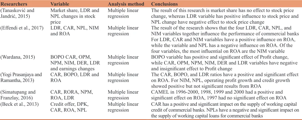
From several studies there are several variables that affect the ROA and Level of Stock Price Changes, which have been summarized as follows in Table 1.
Based on Table 1, there are differences and similarities between research conducted with previous studies. The similarity with the research that will be conducted with some previous research is
to analyze the performance level of banking companies. While
the difference is in the period of study, which for this study used
quarterly periods for 14 periods from March 2004 to June 2007.
In addition, the variables used in this study are capital adequacy ratio, NPL, BOPO, net interest margin (NIM), LDR and ROA.
The emphasis on research using a quantitative approach that is the existence of research framework that is being studied. This notion is based on a philosophy of positivism which says that
symptoms can be classified and symptoms have a causal or causal
relationship.
According to (Vatansever and Hepsen, 2015) definition of the
hypothesis is “a tentative statement that is a conjecture of what
we are observing in an attempt to understand it.”
Based on the writings put forward before the hypothesis proposed is:
H1 : There is the effect of LDR and NPL to ROAs.
H2 : There is influence of ROAs to rate of change of stock price.
H3 : There is the effect of LDR and NPL to the rate of change of stock price.
3. METHODOLOGY
The population of this study are banks listed on the Indonesia
Stock Exchange. The sample of this research is 20 emit or bank
listed in Indonesia Stock Exchange.
LDR This ratio indicates the ability of banks in channeling third party funds collected by the bank concerned. NPLs can be used to measure the extent to which existing problem loans can be met
with the earning assets held by a bank (Makri et al., 2014).
And that being the dependent variable is.
3.1. ROA
This ratio is used to measure the ability of bank assets in obtaining
profit.
3.2. Change of Stock Price
Stocks appeal to investors for various reasons. For some investors, buying stocks is a great way to get big capital (capital gains)
relatively quickly. While for other investors, shares provide income
in the form of dividends.
3.3. Data Analysis
3.3.1. Descriptive statistics a. Mean
Mean is a value that is representative enough for the depiction of the values contained in the data concerned. The formula for the average count of inarched data (ungroup data) is:
1 1
1 n i
X X
n =
=
∑
b. Standard Deviation
The standard deviation are a deviation from the value of the data that has been compiled, and the formula for the standard deviation from the inarched data (ungroup data) is:
2
1
( )
( 1) n
i i
X X
S
n =
− =
−
∑
c. Minimum
Minimum is the smallest value of data.
Table 1: Previous research summary
Researchers Variable Analysis method Conclusions
(Tanasković and
Jandrić, 2015) Market share, LDR and NPL changes in stock price
Multiple linear
regression The result of this research is market share has no effect to stock price change, whereas LDR variable has positive influence to stock price and
NPL change have negative effect to stock price change (Effendiet al., 2017) LDR, CAR, NPL, NIM
and ROA Multiple linear regression The result of the research shows that the four LDR, CAR, NPL, and NIM variables together influence the performance of commercial banks For LDR, CAR and NIM variables have a positive influence on ROA, while the variable and NPL has a negative influence on ROA. Of the four variables, the most influential on ROA are the NIM variable (Wardana, 2015) BOPO CAR, OPM,
NPM, NIM, DER, LDR and earnings changes
Multiple linear
regression BOPO variable has positive and significant effect of Profit change, while CAR, OPM, NPM, NIM, DER and LDR variables have negative
and insignificant effect to Profit change
(Yogi Prasanjaya and
Ramantha, 2013) CAR, BOPO, LDR and ROA Multiple linear regression The CAR, BOPO, and LDR ratios have a positive and significant effect on ROA. For NIM, NPL, operating profit growth and credit growth showed positive but not significant results from ROA
(Simatupang and
Franzlay, 2016) CAR, RORA, NPM, ROA, LDR Multiple linear regression CAMEL in 1996-2000, 1998, 1999 and 2000 had a positive and significant effect on ROA, 1997 had no significant effect on ROA
(Becket al., 2013) Credit offer, DPK,
CAR, ROA, NPL Multiple linear regression CAR has a positive and significant impact on the supply of working capital credit of commercial banks. NPLs have a negative and significant impact on
the supply of working capital loans for commercial banks
d. Maximum
Maximum is the largest value of data.
3.3.2. Test data normality
According to (Niode and Chabachib, 2016) before performing statistical tests the first step that must be done is the screening
of data to be processed. One of the assumptions that the use of parametric statistics is the multivariate normality assumption.
Multivariate normality is the assumption that every variable and all linear combinations of variables are normally distributed. If this assumption is met, then the residual value of the analysis is also normally distributed and independent.
Screening of data normality is a necessary first step for any
multivariate analysis, especially if the goal is inference. That is by looking at the distribution of variables - variables to be studied. Although the normality of a variable is not always required in the analysis but the statistical test results will be better if all variables are normally distributed. If it is not normally distributed (left or right) then the statistical test results will be degraded.
The statistical test that can be used to test data normality is Kolmogorov-Smirnov nonparametric statistical test. K-S test can be done by making hypothesis:
Ho = Data is not normally distributed Ha = Data is normally distributed
With significance level (α) = 5%. If the level of significance is greater than α then the data is normally distributed, but if the level of significance is smaller than α then the data is not normally
distributed.
3.3.3. Classic assumption test
To meet the form of regression models that can be accounted for, there is some classical assumptions that must be met.
3.4. Multicolinearity Test
According to (Niode and Chabachib, 2016) multi collinearity test
aims to test whether the regression model found the correlation between independent variables.
The standard error of the coefficients for the various independent variables are greatly correlated with the coefficient size, so only a small amount of confidence can be placed on the estimated
relationship between each independent variable and the dependent variable. This problem is concerned with multi collinearity, which
is defined as the condition in which independent variables are not
really independent of each other but have values set together. In
SPSS 16.0 for windows program can be tested the presence or
absence of multi collinearity by considering the value of variance
inflation factor (VIF). The result of the Multi collinearity Test is the value of the VIF is <5, and the tolerance value >0.0001.
The formula used to derive VIF values is (Aulia, 2016):
1
= VIF
Tolerance
3.5. Autocorrelation Test
According to (Aulia, 2016) the autocorrelation test aims to test
whether in a linear regression model there is a correlation between the confounding error in period t with the intruder error in period t-1 (previous).
If there is a correlation, it is called an autocorrelation problem. Autocorrelation arises because consecutive observations over time are related to each other. This problem arises because the residual are not free from one observation to another. This is often found
in the time series data because “disturbance” in an individual individual/groups to tends to affect “interference” in the same
individual/group of the next period.
In cross-sectional data, auto correlation problems are relatively
rare because “disturbances” to different observations come
from different individuals/groups. A good regression model is a regression independent of autocorrelation.
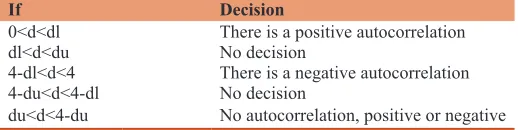
Table 2, the way that can be used in detecting the presence or absence
of autocorrelation Durbin Watson Test, Then the value of DW compared with Durbin Watson table value of the following decision.
3.6. Linearity Test
According to Wibowo and Syaichu (2013) linearity tests is used to see whether the model specifications used are correct or not.
This can be done by plotting between standardized residuals and the estimated value of the standardized dependent variable; which are named scatterplots of residuals. This study uses standardized residuals and predictive values in plots. If there is a relationship
that approximately 95% of residuals lie between -2 and +2 in the
scatterplots of residuals, then the linearity assumption is met.
3.7. Test Heteroscedasticity
According to Zahro and Wahyundaru (2015) heteroscedasticity
test aims to test whether in the regression model there is a variance inequality of the residual one observation to another observation. If the variance between the residual one observation to another observation remains, then it is called heteroscedasticity and if different is called heteroscedasticity. A good model is heteroscedasticity or does not occur heteroscedasticity. Most cross section data contain heteroscedasticity situations because these data collect data representing different sizes.
4. RESULT AND DISCUSSION
4.1. Hypothesis Testing
First hypothesis testing (the influences of LDR and NPL together
to ROAs).
Table 2: Durbin Watson test table
If Decision
0<d<dl There is a positive autocorrelation
dl<d<du No decision
4-dl<d<4 There is a negative autocorrelation
4-du<d<4-dl No decision
du<d<4-du No autocorrelation, positive or negative
1. Multiple correlations
1 2 1 2 1 2
1 2
2 2
2 1 2
2 1
YX YX YX YX X X
YX X
X X
r r r r r
R
r
+ −
=
−
This correlation formula is used to determine the level of relationship between LDR, NPL with ROAs where there are two
variables X and one variables Y.
Table 3, The correlation coefficient value lies between −1 and 1 or −1 ≤ r ≤, if r = 1 then the relationship between variable X and
variable Y is called perfect positive, if r = −1 then the relationship between variable X and variable Y is called the perfect negative
and if r = 0 or close to 0 then the variable X and variable Y have no relationship. In addition, the correlation coefficient also shows
the direction of the relationship.
2. Test of multiple correlation significance
Formulation of hypotheses:
Ho: ρ = 0 (There is no significant relationship between LDR and
NPL with ROAs)
Ha: ρ ≠ 0 (There is a significant relationship between LDR and
NPL with ROAs) test statistics:
1 2
1 2
2
2
/
(1 ) / ( 1)
YX X
YX X
R k
Fo= R n k
− − −
Significant if Fcount > Ftable: H0 rejected
rejected Ftabel: Fα;k;n-k-1
Or significant if the test results of significance <0.05.
3. Multiple linear regression
In this study multiple linear regression analysis is used to see the effect of LDR and NPL together to ROAs.
Ŷ = a+b1X1+b1X2+ε
In this study multiple linear regression analysis is used to see the effect of LDR and NPL together to ROAs:
Ŷ = Subject in the predicted ROAs variable a = Intercept = Value y if X1 and X2 = 0
b = Slope = Number of regression coefficients showing numbers
increases or decrease from dependent variable based on independent variable
X1 = Subject to variable LDR that has a certain value
X2 = Subject to NPL variable that has a certain value
ε = Standard error (standard error of regression).
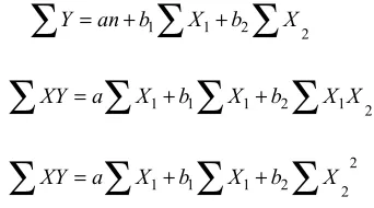
To find value a, b1, b2 then the following equation is used:
∑
Y =an b+ 1∑
X1+b2∑
X21 1 1 2 1 2
XY =a X +b X +b X X
∑
∑
∑
∑
2
1 1 1 2 2
XY =a X +b X +b X
∑
∑
∑
∑
4. Significance Test of Multiple Linear Regression
Formulation of hypotheses:
Ho: β1 = β2 = 0 (There is no significant influence over LDR and
NPL on ROAs)
Ha: β1 ≠ β2 ≠ 0 (There is a significant influence over LDR and
NPL on ROA) Test statistics:
0
/ ( 1)
/ ( )
ESS K
F
RSS N K
−
= −
ESS: Expected sum of square
RSS: Residual sum of square
n: The amount of data
Significant if Fcount > Ftable: H0 rejected
With assumption Ftable:tα;k;n-k-1
Or significant if the test results of significance <0.05.
5. Coefficient of determination
The coefficient of determination is used to find out how far the ability
of the model in explaining the variation of the dependent variables. So
that can know the contribution to LDR and NPL in influencing ROAs.
Calculated by the formula:
KD R= 2YX1 2X x100%
Where:
KD = Coefficient of determination for regression models on LDR
and NPL to ROA YX1 2
R X = Coefficient of multiple correlation LDR, NPL with ROAs.
Based on the results of SPSS processing can be seen the correlation
coefficient between LDR, NPL with ROAs of 0.757, this shows a high and significant relationship between LDR, NPL with ROAs.
Table 3: Interpretation of the magnitude of the correlation coefficient
Coefficient interval Degree of relationship
0.0-199 Very low
0.2-0.399 Low
0.4-0.599 Medium
0.6-0.799 Strong
0.8-1.0 Very strong
Then multiple linear regression equations:
Ŷ = 0.026 + 0.002X1−0.559X2+ε
A constant of 0.026 states that if the LDR and NPL are constant (0), then the ROAs value is 0.026.
Coefficient b1 amounts 0,002 states that each increase in one unit of LDR will decrease ROAs of 0.002.
Coefficient b2 amounts −0,559 states that every increase of one unit of NPL will decrease ROAs of 0.559.
Based on the result of significant regression test it can be seen that with the value of F 35,530 and the significance test value 0.000, it can be concluded that the influence of LDR, NPL to ROAs has a significant influence. In addition ROAs influenced on LDR and NPL of 55.70%, while the rest of 44.30% influenced by other factors.
Based on the results of SPSS processing can be seen the value of
correlation coefficient indicating a positive relationship, very low is not significant between the ROA with Level of Stock Price Changes.
Then the linear regression equation:
Z = 0.128+2.588 X1+ε
Constanta an of 0.128 states that if the ROAs value is constant (0), the value of the Share Price Change Rate is 0.128 units.
The coefficient b of 2588 states that each increase of one unit in ROAs will decrease the Price Change Rate of 2588.
Based on the results of SPSS processing can be seen that the value
of t counts 0.478 is smaller than the value table 2009, it can be concluded that the influence of LDR to ROAs is not significant. While Stock Price Changes Rate is influenced by ROAs of 1.40% while the rest of 93.70% influenced by other factors.
Based on the results of SPSS processing can be seen the value of
correlation coefficient between LDR, NPL with ROAs of 0.126, this indicates a low and insignificant relationship between LDR,
NPL with the rate of stock price changes.
Linear regression equation:
Z = 0.310−0.070X1−3.828X2+ε
Constanta an of 0.310 indicates that if the value of NPL is constant (0), then the value of Change Price Price of 0.310.
The coefficient b1 of −0,070 states every increase of one unit of LDR will decrease the Rate of Change of Stock Price by 0.070.
The coefficient b2 of −3828 states that every increase of one unit
of NPL will decrease the Rate of Change of Stock Price 3828.
While the coefficient of determination of 2.10% means that the rate of change in stock prices is influenced by the NPL of 2.10% while the rest of 97.90% influenced by other factors.
5. CONCLUSION
The results of the test of double correlation significance and non-significant regression due to LDR did not illustrate the extent of current
credit, the amount of npl, and how much bad debts were transferred
to the Indonesian Bank Restructuring Agency. So it does not reflect
income on credit activities and fees on funds raised by banks.
The results of this study are expected to provide input or suggestions to various parties. Based on the results of the study, the authors provide suggestions:
1. Taking into account other factors such as NIM, credit growth, Fee Based Income, Cash Ratio that can affect the ROAs more strongly.
2. Examining the analysis of other financial ratios that can affect
the ROAs is stronger.
Doing research by adding length of observation time, because the longer observation times taken result will be better to take decision.
REFERENCES
Aulia, F. (2016), Pengaruh car, Fdr, Npf, dan bopo terhadap profitabilitas
(return on equity) (Studi empiris pada bank umum syariah di
indonesia periode tahun 2009-2013). Diponegoro Journal of Management, 5(6), 1-10.
Beck, R., Jakubik, P., Piloiu, A. (2013), Non-Performing Loans: What
Matters in Addition to the Economic Cycle? Vol. 6. European Central
Bank Working Paper Series. p12-20.
Effendi, J., Thiarany, U., Nursyamsiah, T. (2017), Factors influencing non-performing financing (NPF) at sharia banking. Walisongo: Jurnal Penelitian Sosial Keagamaan, 25(1), 109-120.
Makri, V., Tsagkanos, A., Bellas, A. (2014), Determinants of non-performing loans: The case of Eurozone. Panoeconomicus, 15(7), 12-21. Niode, N.N., Chabachib, M. (2016), Pengaruh car, pembiayaan, Npf, dan
bopo terhadap roa bank umum syariah di indonesia periode 2010-2015. Diponegoro Journal Of Management, 5(3), 1-13.
Simatupang, A., Franzlay, D. (2016), Capital adequacy ratio(CAR), non performing financing (NPF), efisiensi operasional (BOPO) dan financing to deposit ratio (FDR) terhadap profitabilitas bank umum syariah di Indonesia. Administrasi Kantor, 4(2), 466-485.
Tanasković, S., Jandrić, M. (2015), Macroeconomic and institutional
determinants of non-performing loans. Journal of Central Banking Theory and Practice, 2(8), 23-34.
Vatansever, M., Hepsen, A. (2015), Determining impacts on non-performing loan ratio in Turkey. Journal of Applied Finance and Banking, 9(4), 45-55. Wardana, R.I.P. (2015), Analisis pengaruh CAR, FDR, NPF, BOPO dan
size terhadap profitabilitas pada bank umum syariah di Indonesia (studi kasus pada bank umum syariah di Indonesia periode 2011-2014. Universitas Diponegoro Semarang, 7(1), 67-79.
Wibowo, E.S., Syaichu, M. (2013), Analisis pengaruh suku bunga, inflasi, car, bopo, npf terhadap profitabilitas bank syariah. Diponegoro Journal of Accounting, 2(2), 1-10.
Yogi, P.A.A., Ramantha, I.W. (2013), Analisis pengaruh rasio car, bopo, ldr dan ukuran perusahaan terhadap profitabilitas bank yang terdaftar di bei. Jurnal Akuntansi Universitas Udayana, 41(32), 2302-8556. Zahro, F., Wahyundaru, S.D. (2015), Determinan Kebutuhan Sak Etap
Bagi UKM (Studi Empiris Pada UKM Makanan di Kota Semarang). Vol. 2. 2nd Conference in Business, Accounting, and Management