https://doi.org/10.5194/gmd-12-2727-2019 © Author(s) 2019. This work is distributed under the Creative Commons Attribution 4.0 License.
Description and basic evaluation of simulated mean state, internal
variability, and climate sensitivity in MIROC6
Hiroaki Tatebe1, Tomoo Ogura2, Tomoko Nitta3, Yoshiki Komuro1, Koji Ogochi1, Toshihiko Takemura4,
Kengo Sudo5, Miho Sekiguchi6, Manabu Abe1, Fuyuki Saito1, Minoru Chikira3, Shingo Watanabe1, Masato Mori7, Nagio Hirota2, Yoshio Kawatani1, Takashi Mochizuki1, Kei Yoshimura3, Kumiko Takata2, Ryouta O’ishi3,
Dai Yamazaki8, Tatsuo Suzuki1, Masao Kurogi1, Takahito Kataoka1, Masahiro Watanabe3, and Masahide Kimoto3 1Research Center for Environmental Modeling and Application, Japan Agency for Marine-Earth Science and Technology, 3173-25 Showamachi, Kanazawaku, Yokohama, Kanagawa 236-0001, Japan
2National Institute for Environmental Studies, Tsukuba, Japan
3Atmosphere and Ocean Research Institute, University of Tokyo, Kashiwa, Japan 4Research Institute for Applied Mechanics, Kyushu University, Kasuga, Japan 5Graduate School of Environmental Studies, Nagoya University, Nagoya, Japan 6Tokyo University of Marine Science and Technology, Tokyo, Japan
7Research Center for Advanced Science and Technology, University of Tokyo, Tokyo, Japan 8Institute of Industrial Sciences, University of Tokyo, Tokyo, Japan
Correspondence:Hiroaki Tatebe ([email protected]) Received: 23 June 2018 – Discussion started: 16 July 2018
Revised: 15 May 2019 – Accepted: 31 May 2019 – Published: 8 July 2019
Abstract. The sixth version of the Model for Interdisci-plinary Research on Climate (MIROC), called MIROC6, was cooperatively developed by a Japanese modeling community. In the present paper, simulated mean climate, internal cli-mate variability, and clicli-mate sensitivity in MIROC6 are eval-uated and briefly summarized in comparison with the pre-vious version of our climate model (MIROC5) and obser-vations. The results show that the overall reproducibility of mean climate and internal climate variability in MIROC6 is better than that in MIROC5. The tropical climate systems (e.g., summertime precipitation in the western Pacific and the eastward-propagating Madden–Julian oscillation) and the midlatitude atmospheric circulation (e.g., the westerlies, the polar night jet, and troposphere–stratosphere interactions) are significantly improved in MIROC6. These improvements can be attributed to the newly implemented parameterization for shallow convective processes and to the inclusion of the stratosphere. While there are significant differences in cli-mates and variabilities between the two models, the effective climate sensitivity of 2.6 K remains the same because the dif-ferences in radiative forcing and climate feedback tend to offset each other. With an aim towards contributing to the
sixth phase of the Coupled Model Intercomparison Project, designated simulations tackling a wide range of climate sci-ence issues, as well as seasonal to decadal climate predic-tions and future climate projecpredic-tions, are currently ongoing using MIROC6.
1 Introduction
2728 H. Tatebe et al.: Basic evaluation of MIROC6
continental regions (e.g., Church and White, 2011; Bamber and Aspinall, 2013). Additionally, ocean acidification due to the absorption of atmospheric carbon dioxide (CO2) and changes in carbon–nitrogen cycles are expected to lead to the loss of Earth biodiversity (e.g., Riebesell et al., 2009; Rock-ström et al., 2009; Taucher and Oschlies, 2011; Watanabe and Kawamiya, 2017). Societal demands for information on global and regional climate changes have increased signifi-cantly worldwide in order to meet information requirements for political decision-making related to mitigation and adap-tation to global warming.
The Intergovernmental Panel on Climate Change (IPCC) has continuously published assessment reports (ARs) in which a comprehensive view of past, present, and future climate changes on various timescales, including centen-nial global warming, is synthesized. Together with obser-vations, climate models have been contributing to the IPCC ARs through a broad range of numerical simulations, espe-cially future climate projections after the twenty-first century. However, there are many uncertainties in future climate pro-jections, and the range of uncertainties has not been narrowed by an update of the IPCC reports. The uncertainties are aris-ing from imperfections of climate models in representaris-ing mi-croscale to global-scale physical and dynamical processes in subsystems of the Earth’s climate and their interactions. To reduce the uncertainties and errors in climate projections and predictions, utilizing observations, extracting the essences of physical processes in the real climate, and investigating the response of the climate system to various external forcings based on a set of climate model simulations are necessary. In particular, a state-of-the-art climate model that can represent various processes in the Earth’s climate system is a powerful tool for a deeper understanding of the Earth’s climate system. One Japanese climate model, which is called MIROC (Model for Interdisciplinary Research on Climate), has been cooperatively developed at the Center for Climate System Research (CCSR; the precursor of a part of the Atmosphere and Ocean Research Institute), the University of Tokyo, the Japan Agency for Marine-Earth Science and Technol-ogy (JAMSTEC), and the National Institute for Environmen-tal Studies (NIES). Utilizing MIROC, our Japanese climate modeling group has been tackling a wide range of climate science issues as well as seasonal to decadal climate predic-tions and future climate projecpredic-tions. At the same time, by providing simulation data, we have been participating in the third and fifth phases of the Coupled Model Intercompari-son Project (CMIP3 and CMIP5; Meehl et al., 2007; Taylor et al., 2012) that has been contributing to the IPCC ARs by synthesizing multi-model ensemble datasets.
In the years up to the IPCC fifth assessment report (IPCC AR5; IPCC, 2013), we have developed four versions of MIROC, three of which (MIROC3m, MIROC3h, and MIROC4h) have almost the same dynamical and physical packages but different resolutions. MIROC3m (K-1 model developers, 2004) is composed of T42L20 atmosphere and
1.4◦L43 ocean. Resolutions of MIROC3h (K-1 model devel-opers, 2004) are higher than MIROC3m and are T106L56 for the atmosphere and eddy-permitting for the ocean (1/4◦× 1/6◦). Only the horizontal resolution of the atmosphere of MIROC3h is changed to T213 in MIROC4h (Sakamoto et al., 2012). MIROC5 is composed of T85L40 atmosphere and 1.4◦L50 ocean but with considerably updated physical and dynamical packages (Watanabe et al., 2010). These mod-els have been used to study various scientific issues such as the detection of natural influences on climate changes (e.g., Nozawa et al., 2005; Mori et al, 2014; Watanabe et al., 2014), uncertainty quantification of climate sensitivity (e.g., Shiogama et al., 2012; Kamae et al., 2016), future pro-jections of regional sea level rises (e.g., Suzuki et al., 2005; Suzuki and Ishii, 2011), and mechanism studies on tropical decadal variability (e.g., Tatebe et al., 2013; Mochizuki et al., 2016).
essen-tial for better representing observed climatic mean states and internal climate variability. In addition to physical parameter-izations, enhanced vertical resolution in both atmosphere and ocean components, along with a highly accurate tracer ad-vection scheme, has been suggested to have impacts on the reproducibility of model climate and internal climate vari-ations (e.g., Tatebe and Hasumi, 2010; Ineson and Scaife, 2009; Scaife et al., 2012).
Recently, we have developed the sixth version of MIROC, called MIROC6. This newly developed climate model has updated physical parameterizations in all sub-modules. In or-der to suppress an increase in computational cost, the hor-izontal resolutions of MIROC6 are not significantly higher than those of MIROC5. The reason is that a larger number of ensemble members is required to realize significant sea-sonal predictions of, for example, the wintertime Eurasian climate (Murphy, 1990; Scaife et al., 2014). Indeed, climate predictions by the older versions of MIROC having at most 10 ensemble members are skillful only in the tropical climate and the midlatitude ocean, not in the midlatitude atmosphere. Large-ensemble predictions are also required in decadal-scale predictions in order to evaluate the human influences on near-term climate changes. The model top in MIROC6 is placed at the 0.004 hPa pressure level, which is higher than that of MIROC5 (3 hPa), and the stratospheric vertical reso-lution has been enhanced in comparison to MIROC5 in or-der to represent the stratospheric circulation. Overall, the re-producibility of the mean climate and internal variability of MIROC6 is better than that of MIROC5, but the model’s computational cost is about 3.6 times as large as that of MIROC5. Considering that the computational costs of large-ensemble predictions based on climate models with horizon-tal resolutions of, for example, 50 km atmosphere and eddy-resolving ocean are still huge on recent computer systems, the use of relatively low-resolution models such as MIROC6 with further elaborated parameterizations can still be actively useful in science-oriented climate studies and climate predic-tions produced for societal needs.
The rest of the present paper is organized as follows. We describe the model configuration, tuning, and spin-up procedures in Sect. 2, while simulated mean state, internal variability, and climate sensitivity are evaluated in Sect. 3. Simulation performance of MIROC6 and remaining issues are briefly summarized and discussed in Sect. 4. Currently, MIROC6 is being used for various simulations designed by the sixth phase of CMIP (CMIP6; Eyring et al., 2016), which aims to strengthen the scientific basis of IPCC AR6. Large-ensemble simulations and climate predictions using MIROC6 are also ongoing for science-oriented studies in our modeling group and for societal benefits. In addition, the lat-est Earth system model version of MIROC with the global carbon cycle, whose physical core will be MIROC6, has been developed for CMIP6 towards a further wide range of is-sues regarding climate and societal applications (Hajima et al., 2019).
2 Model configurations and spin-up procedures MIROC6 is composed of three sub-models: atmosphere, land, and sea ice–ocean. The atmospheric model is based on the CCSR-NIES atmospheric general circulation model (AGCM; Numaguti et al., 1997). The land surface model is based on Minimal Advanced Treatments of Surface Interac-tion and Runoff (MATSIRO; Takata et al. 2003), which in-cludes a river-routing model from Oki and Sud (1998) based on a kinematic wave flow equation (Ngo-Duc et al., 2007) and a lake module in which one-dimensional thermal dif-fusion and mass conservation are considered. The sea ice– ocean model is based on the CCSR Ocean Component model (COCO; Hasumi, 2006). A coupler system calculates heat and freshwater fluxes between the sub-models in order to en-sure that all fluxes are conserved within machine precision and then exchanges the fluxes among the sub-models (Suzuki et al., 2009). No flux adjustments are used in MIROC6. In the remaining part of this section, we will provide de-tails on MIROC6 configurations, focusing on updates from MIROC5. Readers may also refer to Table A1 in Appendix A where the updates are briefly summarized.
2.1 Atmospheric component
MIROC6 employs a spectral dynamical core in its AGCM component as in MIROC5. The horizontal resolution is a T85 spectral truncation that is an approximately 1.4◦grid interval for both latitude and longitude. The vertical grid coordinate is a hybridσ–pcoordinate (Arakawa and Konor, 1996). The model top is placed at 0.004 hPa, and there are 81 vertical levels (Fig. 1a). The vertical grid arrangement in MIROC6 is considerably enhanced in comparison to that in MIROC5 (40 levels; 3 hPa) so that the stratospheric circulation can be rep-resented. A sponge layer that damps wave motions is set at the model-top level by increasing Rayleigh friction to prevent extra wave reflection near the model top. The atmospheric component of MIROC6 has standard physical parameteriza-tions for cumulus convection, radiation transfer, cloud mi-crophysics, turbulence, and gravity wave drag. It also has an aerosol module. These are basically the same as those used in MIROC5, but several updates have been made, as will be de-tailed below. The parameterizations for cloud microphysics and planetary boundary layer processes in MIROC6 are the same as in MIROC5. The standard time step for MIROC6 is 6 min, which is shorter than that of MIROC5 (12 min) be-cause stratospheric winds whose speed sometimes exceeds 150 m s−1must be resolved in time integration. The time step for radiative transfer models is set separately and is 3 h in both MIROC6 and MIROC5.
2730 H. Tatebe et al.: Basic evaluation of MIROC6
Figure 1. Vertical half-levels for the atmospheric (a) and the oceanic(b)components of MIROC6 and MIROC5.
however, tends to overestimate low-level cloud amounts over the low-latitude oceans and has a dry bias in the free tro-posphere. These biases appear to be the result of insuffi-cient vertical mixing of the humid air in the planetary bound-ary layer and the dry air in the free troposphere. To allevi-ate these biases, an additional parameterization for shallow cumulus convection based on Park and Bretherton (2009) is implemented in MIROC6. Shallow convection associated with atmospheric instability is calculated by the Chikira and Sugiyama (2010) scheme, and that associated with turbu-lence in the planetary boundary layer is represented by the Park and Bretherton (2009) scheme. The shallow convective parameterization is a mass flux scheme based on a buoyancy-sorting, entrainment–detrainment, single-plume model that calculates the vertical transport of liquid water, potential tem-perature, total water mixing ratio, and horizontal winds in the lower troposphere. The cloud-base mass flux is controlled by turbulent kinetic energy within the sub-cloud layer and convective inhibition. The cloud-base height for shallow cu-mulus is set between the lifting condensation level and the boundary layer top, which is diagnosed based on the vertical profile of relative humidity. When implementing the param-eterization in MIROC6, the following conditions for trigger-ing the shallow convection are specified: (1) the estimated inversion strength (Wood and Bretherton, 2006) is smaller than a tuning parameter, and (2) the convection depth diag-nosed by a separate cumulus convection scheme (Chikira and Sugiyama, 2010) is smaller than a tuning parameter.
The Spectral Radiation Transport Model for Aerosol Species (SPRINTARS; Takemura et al., 2000, 2005, 2009) is used as an aerosol module for MIROC6 to predict the mass mixing ratios of the main tropospheric aerosols, which are black carbon, organic matter, sulfate, soil dust, sea salt, and the precursor gases of sulfate (sulfur dioxide, SO2,
and dimethylsulfide). By coupling the radiation and cloud– precipitation schemes in MIROC, SPRINTARS calculates not only the aerosol transport processes of emission, advec-tion, diffusion, sulfur chemistry, wet deposiadvec-tion, dry deposi-tion, and gravitational settling, but also the aerosol–radiation and aerosol–cloud interactions. There are two primary up-dates in SPRINTARS of MIROC6 that were not included in MIROC5. One is the treatment of precursor gases of or-ganic matter as prognostic variables. In the previous version, the conversion rates from the precursor gases (e.g., terpene and isoprene) to organic matter are prescribed (Takemura et al., 2000), while an explicit simplified scheme for secondary organic matter was introduced from a global chemical cli-mate model (Sudo et al., 2002). The other is a treatment of oceanic primary and secondary organic matter. Emissions of primary organic matter are calculated with wind at a 10 m height, the particle diameter of sea salt aerosols, and chloro-phyllaconcentration at the ocean surface (Gantt et al., 2011). The oceanic isoprene and monoterpene, which are precursor gases of organic matter, are emitted depending on the photo-synthetically active radiation, diffuse attenuation coefficient at 490 nm, and the ocean surface chlorophyllaconcentration (Gantt et al., 2009).
The radiative transfer in MIROC6 is calculated by an up-dated version of thek-distribution scheme used in MIROC5 (Sekiguchi and Nakajima, 2008). The single-scattering pa-rameters have been calculated and tabulated in advance, and liquid, ice, and five aerosol species can be treated in this up-dated version. Given the significant effect of crystal habit on a particle’s optical characteristics (Baran, 2012), the assump-tion of ice particle habit has been updated from our previous simple assumption of a sphere used in MIROC5 to a hexago-nal solid column (Yang et al., 2013) in MIROC6. The upper limits of the mode radius of cloud particles have been ex-tended from 32 µm to 0.2 mm for liquids and from 80 µm to 0.5 mm for ice. Therefore, the scheme can now handle the large-sized water particles (e.g., drizzle and rain) that have been shown to have significant radiative impacts (Waliser et al., 2011).
middle atmosphere circulation, frequency of sudden strato-spheric warmings, and period and amplitude of the equatorial quasi-biennial oscillations (QBOs) can be represented.
2.2 Land surface component
The land surface model is also basically the same as in MIROC5. Energy and water exchanges between land and at-mosphere are calculated, considering the physical and phys-iological effects of vegetation with a single-layer canopy, as well as the thermal and hydrological effects of snow and soil, respectively, with three-layer snow and six-layer soil down to a 14 m depth. Sub-grid fractions of land use and snow cover have also been considered. The time step for the land surface model integration is 1 h in MIROC6, which is the same as in MIROC5. In addition to the standard package in MIROC5, a few other physical parameterizations are implemented as described below.
A physically based parameterization of sub-grid snow dis-tribution (SSNOWD; Liston, 2004; Nitta et al., 2014) re-places the simple functional approach of snow water equiv-alent in calculating sub-grid snow fractions in MIROC5 in order to improve the seasonal cycle of snow cover. In SS-NOWD, the snow cover fraction is formulated for accumu-lation and abaccumu-lation seasons separately. For the abaccumu-lation sea-son, the snow cover fraction decreases based on the sub-grid distribution of the snow water equivalent. A lognormal dis-tribution function is assumed and the coefficient of variation category is diagnosed from the standard deviation of the sub-grid topography, coldness index, and vegetation type that is a proxy for surface winds. While the cold degree month was adopted for coldness in the original SSNOWD, we decided instead to introduce the annually averaged temperature over the latest 30 years using the time relaxation method of Krin-ner et al. (2005), in which the timescale parameter is set to 16 years. The temperature threshold for a category diagno-sis is set to 0 and 10◦C. In addition, a scheme represent-ing a snow-fed wetland that takes into consideration sub-grid terrain complexity (Nitta et al., 2017) is incorporated. The river-routing model and lake module are the same as those used in MIROC5, but the river network map is updated to keep the consistency with the new land–sea mask (Yamazaki et al., 2009).
2.3 Ocean and sea ice component
The ocean component of MIROC6 is basically the same as that used in MIROC5, but several updates are implemented as described below. The warped bipolar horizontal coordi-nate system in MIROC5 has been replaced by the tripolar coordinate system proposed by Murray (1996). Two singu-lar points in the biposingu-lar region to the north of about 63◦N are placed at (63◦N, 60◦E) in Canada and (63◦N, 120◦W) in Siberia (Fig. 2). In the spherical coordinate portion to the south of 63◦N, the longitudinal grid spacing is 1◦ and
Figure 2.Horizontal grid coordinate system and model bathymetry of the ocean component of MIROC6.
the meridional grid spacing varies from about 0.5◦near the Equator to 1◦in the midlatitudes. In the central Arctic Ocean where the bipole coordinate system is applied, the grid spac-ings are about 60 km zonal and 33 km meridional, respec-tively. By introducing the horizontal tripolar coordinate sys-tem, it is expected that theoretical westward propagation of the oceanic baroclinic Rossby can be represented with fewer numerical dispersions because of agreement of the coordi-nate system and the geographical coordicoordi-nate system. It is also expected that the horizontal resolutions in the Arctic Ocean where the Rossby radius of deformation is relatively small are higher than in the case in which the bipolar warped coor-dinate system in MIROC5 is adopted. There are 62 vertical levels in a hybridσ–zcoordinate system. The horizontal grid spacing in MIROC5 is nominally 1.4◦, except for the equa-torial region, and there are 49 vertical levels. The resolutions in MIROC6 are higher than in MIROC5. In particular, 31 (23) of the 62 (49) vertical layers in MIROC6 (MIROC5) are within the upper 500 m of depth (Fig. 1b). The increased number of vertical layers in MIROC6 has been adopted in order to better represent the equatorial thermocline and ob-served complex hydrography in the Arctic Ocean. An in-crease in computational costs of the ocean component due to higher resolutions in MIROC6 is suppressed by implement-ing a time-staggered scheme for the tracer and baroclinic mo-mentum equations (Griffies et al., 2005). Owing to the time-staggered scheme, the time step for the ocean and sea ice components of MIROC6 is 20 min, which is longer than that in MIROC5 (15 min).
de-2732 H. Tatebe et al.: Basic evaluation of MIROC6
termined in the same manner as that of MIROC5, except for the Arctic region. An empirical profile of background ver-tical diffusivity, which is proposed in Tsujino et al. (2000), is modified above the 50 m depth to the north of 65◦N. It is 1.0×10⁻⁶m2s−1 in the uppermost 29 m and gradually increases to 1.0×10⁻⁵m2s−1at the 50 m depth. Addition-ally, the turbulent mixing process in the surface mixed layer is changed so that there is no surface wave breaking and no resultant near-surface mixing in regions covered by sea ice. The combination of the weak background vertical diffusivity and suppression of turbulent mixing under the sea ice con-tributes to better representations of the surface stratification in the Arctic Ocean with little impact on the rest of the global oceans (Komuro, 2014).
The sea ice component in MIROC6 is almost the same as in MIROC5. A brief description, along with some ma-jor parameters, is given here. Readers may refer to Komuro et al. (2012) and Komuro and Suzuki (2013) for further de-tails. A sub-grid-scale sea ice thickness distribution is incor-porated by following Bitz et al. (2001). There are five ice categories (plus one additional category for open water), and the lower bounds of the ice thickness for these categories are set to 0.3, 0.6, 1, 2.5, and 5 m. The momentum equation for sea ice dynamics is solved using elastic–viscous–plastic rhe-ology (Hunke and Dukowicz, 1997). The strength of the ice per unit thickness and concentration is set at 2.0×10⁴N m−2, and the ice–ocean drag coefficient is set to 0.02. The sur-face albedo for bare ice sursur-face is 0.85 (0.65) for the visible (infrared) radiation. The surface albedo in snow-covered ar-eas is 0.95 (0.80) when the surface temperature is lower than
−5◦C for the visible (infrared) radiation, and it is 0.85 (0.65) when the temperature is 0◦C. Note that the albedo changes linearly between−5 and 0◦C. These parameter values listed here are the same as those listed in MIROC5.
2.4 Boundary conditions
A set of external forcing data recommended by the CMIP6 protocol is used. The historical solar irradiance spectra, greenhouse gas concentrations, anthropogenic aerosol emis-sions, and biomass burning emissions are given by Matthes et al. (2017), Meinshausen et al. (2017), Hoesly et al. (2018), and van Marle et al. (2017), respectively. The concentra-tions of greenhouse gases averaged globally and annually are given to MIROC6. Radiative forcing of stratospheric aerosols due to volcanic eruptions is computed by verti-cally integrating extinction coefficients for each radiation band, which are provided by Thomason et al. (2019), in the model layers above the tropopause. Three-dimensional at-mospheric concentrations of historical ozone (O3) are pro-duced by the Chemistry–Climate Model Initiative (Hegglin et al., 2019; the data are available at http://blogs.reading. ac.uk/ccmi/forcing-databases-in-support-of-cmip6/, last ac-cess: 6 July 2016). Three-dimensional concentrations of the OH radical, hydrogen peroxide (H2O2), and nitrate (NO3)
are precalculated by a chemical atmospheric model from Sudo et al. (2002). As precursors of secondary organic aerosol, emission data on terpenes and isoprene provided by the Global Emissions Inventory Activity (Guenther et al., 1995) are normally used, although simulated emissions from the land ecosystem model of Ito and Inatmoni (2012) are also used alternatively.
For specifying the soil types and area fractions of natural vegetation and cropland on grids of the land surface com-ponent, the harmonized land use dataset (Hurtt et al., 2011), Center for Sustainability and the Global Environment global potential vegetation dataset (Ramankutty and Foley, 1999), and the dataset provided by the International Satellite Land Surface Climatology Project Initiative I (Sellers et al., 1996) are used. These datasets are also used in prescribing back-ground reflectance at the land surface. Leaf area index data are prepared based on the moderate-resolution imag-ing spectroradiometer leaf area index products of Myneni et al. (2002).
The forcing dataset used for the preindustrial control simu-lation is basically composed of data for the year 1850, which are included in the abovementioned historical dataset. The stratospheric aerosols and solar irradiance in the preindus-trial simulation are given as monthly climatology averaged in 1850–2014 and in 1850–1873, respectively. The total so-lar irradiance is about 1361 W m−2, and the global mean con-centrations of CO2, methane (CH4), and nitrous oxide (N2O) are 284.32 ppm, 808.25 ppb, and 273.02 ppb, respectively.
2.5 Spin-up and tuning procedures
components are coupled with the ocean component. Surface topography in the atmospheric and land surface component is also made using the ETOPO5 dataset. Note that the hori-zontal grid arrangement of the land surface model is exactly the same as the atmospheric component. The coupling in-terval among the sub-models is 1 h. An initial condition of the ocean component in MIROC6 is given by the stand-alone ocean experiment, and those of the atmosphere and land are taken from an arbitrary year of the preindustrial control run of MIROC5.
After coupling the sub-models, climate model tuning is done under the preindustrial boundary conditions. Conven-tionally, the climate models of our modeling community are retuned in coupled modes after stand-alone sub-model tun-ing. This is because the reproducibility of climatic mean state and internal climate variations is not necessarily guaranteed in climate models with the same parameters determined in stand-alone sub-model tuning, which is particularly the case in the tropical climate. In our tuning procedures described below, many of the 10-year-long climate model runs are con-ducted with different parameter values. There are numer-ous parameters associated with physical parameterizations, whose upper–lower bounds are constrained by empirical or physical reasoning. The main parameters used in our tuning procedures are chosen by referring to a perturbed parame-ter ensemble set made by Shiogama et al. (2012) in which parameter sensitivity to cloud radiative processes is exam-ined. The impact of parameter tuning on the present climate is also discussed by Ogura et al. (2017), focusing on top-of-atmosphere (TOA) radiation and clouds. Any objective and optimal methods for parameter tuning are not used in our modeling group, and the tuning procedures are like those in other climate modeling groups as summarized in Hourdin et al. (2017).
In the first model tuning step, climatology, seasonal pro-gression, and internal climate variability in the tropical cou-pled system are tuned so that departures from observations or reanalysis datasets are reduced. Here, it should be noted that representation of the tropical system in MIROC6 is sensi-tive to the parameters for convection and planetary boundary layer processes. Specifically, parameters of reference height for cumulus precipitation, efficiency of the cumulus entrain-ment of the surrounding environentrain-ment, and maximum cumu-lus updraft velocity at the cumucumu-lus base are used to tune the strength of the equatorial trade wind, the climatologi-cal position and intensity of the Intertropiclimatologi-cal Convergence Zone (ITCZ) and South Pacific Convergence Zone (SPCZ), and the interannual variability of the El Niño–Southern Os-cillation (ENSO). In particular, the parameter for the cumu-lus entrainment is known as a controlling factor of ENSO in MIROC5 (Watanabe et al., 2011). Summertime precipitation in the western tropical Pacific that is characteristic of tropical intra-seasonal oscillations is tuned by using the parameter for shallow convection describing the partitioning of turbulent kinetic energy between horizontal and vertical motions at the
sub-cloud layer inversion. Next, the wintertime midlatitude westerly jets and the stationary waves in the troposphere are tuned using the parameters of the orographic gravity wave drag and the hyper-diffusion of momentum. The parameters of the hyper-diffusion and the non-orographic gravity wave drag are also used when tuning stratospheric circulation of the polar vortex and QBO. Finally, the radiation budget at the TOA is tuned, primarily using the parameters for the auto-conversion process so that excess downward radiation can be minimized and maintained closer to 0.0 W m−2. The surface albedos for bare sea ice and snow-covered sea ice are set to higher values than in observations (see Sect. 2.3) in order to avoid underestimating the summertime sea ice extent in the Arctic Ocean due to excess downward shortwave radiation in this region. In addition, parameter tuning for the total radia-tive forcing associated with aerosol–radiation and aerosol– cloud interactions is done. So that the total radiative forcing can be closer to the estimate of−0.9 W m−2 (IPCC, 2013; negative value indicates cooling) with an uncertainty range of
−1.9 to−0.1 W m−2, parameters of cloud microphysics and the aerosol transport module, such as the timescale for cloud droplet nucleation, in-cloud properties of aerosol removal by precipitation, and the minimum threshold for the number concentration of cloud droplets, are perturbed. To determine a suitable parameter set, several pairs of a present-day run under the anthropogenic aerosol emissions at the year 2000 and a preindustrial run are conducted. A pair of present and preindustrial runs has exactly the same parameters, and dif-ferences of tropospheric radiation between two runs are con-sidered anthropogenic radiative forcing. Note that MIROC6 in a coupled mode is used in this tuning procedure, and thus the sea surface temperature (SST) is not fixed. The estimated radiative forcing here is not strictly the same as the effective radiative forcing estimated in IPCC (2013). However, by the present tuning procedure, the global mean surface air temper-ature (SAT) change after the mid-nineteenth century is well reproduced in the historical runs by MIROC6 (details are dis-cussed in Sect. 4). As mentioned above, the reproducibility of the global mean SAT is not a tuning goal but is a typi-cal metric that reflects results of the parameter tunings for individual processes of convection, dynamics, and radiative forcing.
2734 H. Tatebe et al.: Basic evaluation of MIROC6
Figure 3. (a)Time series of the global mean SAT (solid) and the TOA radiation budget (dashed; upward positive).(b)Same as(a), but for the global mean SST (solid) and the ocean temperature through the full water column (dashed).
Figure 3 shows the time series of the global mean quanti-ties after the spin-up. The labeled year in Fig. 3 indicates the elapsed year after the spin-up duration of 2000 years. The lin-ear trend of the global mean SAT is 9.5×10⁻³K per century and is much smaller than the observed value of about 0.62 K per century in the twentieth century, indicating that there is no significant drift and the global mean SAT is in a quasi-steady state. While the global mean SST is in a quasi-quasi-steady state (linear trend of 7.0×10⁻³K per century), the global mean ocean temperature shows a larger trend of 6.8×10⁻³K per century in the first 500 years than that of 1.3×10⁻³K per century in the later period. In the later sections, the 200-year-long data between the 500th and 699th years are analyzed.
The trend of the global mean ocean temperature in the later period suggests slight but continuous warming of the deep ocean. The radiation budget at the TOA is 1.1 W m−2 downward on average (linear trend of 9.5×10⁻³K per cen-tury), and the net heat input at the sea surface is 0.32 W m−2. The deep ocean warming is explained by the net heat in-put. Note that there is about 0.78 W m−2of inconsistency be-tween the TOA radiation budget and the ocean heat uptake. This heat energy inconsistency is due to internal energy as-sociated with precipitation, water vapor, and river runoff not being taken account in the atmospheric and land surface com-ponent in MIROC6, as well as the fact that these waters with no temperature information implicitly set their temperature to the SST when they flow or fall into the ocean. Perpetual melting of the prescribed Antarctic ice sheet with invariant
Table 1.Summary of observation and reanalysis datasets used as references in the present paper.
Dataset Data Reference
period (year)
CERES (edition 2.8) 2001–2013 Loeb et al. (2009) ISCCP Climatology Zhang et al. (2004) ERA-Interim 1980–2009 Dee et al. (2011) GPCPv2 1980–2009 Adler et al. (2003)
EASE-Grid 2.0 1980–2009 Brodzik and Armstrong (2013) ProjD 1980–2009 Ishii et al. (2003)
SODA 1980–2009 Carton and Giese (2008) SSM/I 1980–2009 Cavarieli et al. (1991) NOAA OLR 1974–2013 Liebmann and Smith (1996) COBE-SST2–SLP2 1900–2013 Hirahara et al. (2014) HadCRUT 1850–2015 Morice et al. (2012)
ice thickness, which occurs due to the warm SAT bias in the Antarctic region (details will be discussed in Sect. 3.1.3), is also a cause of the heat energy inconsistency.
3 Results of preindustrial simulation
Representations of climatic mean field and internal climate variability in MIROC6 (Tatebe and Watanabe, 2018a) are evaluated in comparison with MIROC5 and observations. The 200-year-long data of the preindustrial control simula-tion by MIROC5 are used. The observasimula-tions and reanalysis datasets used in the comparison are listed in Table 1.
Here, the model climatology in the preindustrial simu-lations is compared with observations in recent decades. Because observations are obtained concurrently with the progress of global warming due to increasing anthropogenic radiative forcing, the model climate under preindustrial con-ditions may not be adequate for use when making com-parisons with recent observations. However, the root mean squared (RMS) errors of typical variables (e.g., the global mean SAT) in the climate models with respect to observa-tions are much larger than the RMS differences between the model climatology in the preindustrial simulation and those in the last 30-year-long period in the historical simula-tions. Therefore, the differences between the time periods for which the climatology is defined are not a significant concern in comparisons among the climate models and observations. 3.1 Climatology
3.1.1 Atmosphere and land surface
data are available at https://ceres.larc.nasa.gov/, last access: 12 June 2018). At the top right of each panel, a global mean (GM) value and a root mean squared error (RMSE) with re-spect to observations are written. In the present paper, RMSE is computed without model and observed global mean quan-tities unless otherwise noted.
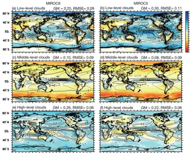
Persistent overestimates of net shortwave radiative flux and the sum of net shortwave and net longwave fluxes over low-latitude oceans in MIROC5 are significantly reduced in MIROC6. Hereafter, net shortwave radiation, net long-wave radiation, and their sum are denoted as OSR, OLR, and NET, respectively, for simplicity. As described in Ogura et al. (2017), since parameter tuning cannot eliminate the abovementioned excess upward radiation, it is suggested that implementing a shallow convective parameterization is re-quired in order to reduce the biases. Figure 5 shows annual mean moistening rates associated with deep and shallow con-vection at the 850 hPa pressure level in MIROC6. Moisten-ing due to shallow convection occurs mainly over the low-latitude oceans, especially the eastern subtropical Pacific and the western Atlantic and Indian oceans. These active regions of shallow convection occur separately from regions with active deep convection in the western tropical Pacific and the ITCZ. The clear separation of the two convection types is consistent with satellite-based observations (Williams and Tselioudis, 2007). Owing to the shallow convective process that mixes the humid air in the planetary boundary layer with the dry air in the free troposphere, low-level cloud cover over the low-latitude oceans is better represented in MIROC6 than in MIROC5. Figure 6 shows annual mean biases in cloud covers with respect to the International Satellite Cloud Cli-matology Project (ISCCP; Rossow et al., 1996; Zhang et al., 2004; the data are available at https://isccp.giss.nasa.gov/, last access: 26 February 2018). An overestimate of low-level cloud cover over the low-latitude oceans in MIROC5 (Fig. 6b) is apparently reduced in MIROC6 (Fig. 6a), which results in smaller NET and OSR biases (Fig. 4). RMS error in low-level cloud cover in MIROC6 is 9 % lower than that in MIROC5.
OSR in the midlatitudes is also better represented in MIROC6 than in MIROC5. Zonally distributed downward OSR bias in MIROC5 is reduced or becomes a relatively small upward bias in MIROC6 (Fig. 4c, d). This differ-ence in the OSR bias is commonly found in both hemi-spheres. Cloud cover at middle and high levels is larger in MIROC6 over the subarctic North Pacific, North Atlantic, and the Southern Ocean (Fig. 6c–f), while low-level cloud cover over the same regions is smaller in MIROC6 than in MIROC5 over the same regions (Fig. 6a, b). The smaller low-level cloud cover in MIROC6 is inconsistent with the larger upward OSR bias in MIROC6. The wintertime midlatitude westerlies are stronger and are located more poleward in MIROC6 than in MIROC5. Correspondingly, the activity of sub-weekly disturbances in the midlatitudes is strengthened in MIROC6 (details are described later). These differences
in the midlatitude atmospheric circulation between MIROC6 and MIROC5 lead to an enhanced poleward moist air trans-port from the subtropics to the subarctic region, which could result in an increase in the mid- and high-level cloud cover in MIROC6, as reported in previous modeling studies (e.g., Bodas-Salcedo et al., 2012; Williams et al., 2013). Con-sequently, the downward OSR bias in the midlatitudes is smaller in MIROC6 than in MIROC5. In polar regions, both biases in OSR and NET remain the same as in MIROC5.
Systematic bias in the outgoing longwave radiative flux (hereafter OLR) is worse in MIROC6 than in MIROC5 be-cause MIROC6 tends to underestimate OLR over almost the entire global domain, except for Antarctica (Fig. 4e, f). The global mean of the high-level cloud cover in MIROC6 is larger than in MIROC5 by 0.04 (Fig. 6e, f), which is con-sistent with the smaller OLR in MIROC6. The increased moisture transport due to the strengthening of the westerlies and sub-weekly disturbances can partly explain the increase in the midlatitude level clouds in MIROC6, but high-level cloud cover is also larger in the low latitudes. Hirota et al. (2018) reported that moistening of the free troposphere due to shallow convection creates favorable conditions for atmospheric instabilities that lead to the resultant activation of deep convection at the low latitudes. Such processes may contribute to the inferior representation of OLR in MIROC6. Next, we will discuss the global budget of the radiative fluxes and the RMS errors between models and observa-tions. Note that only deviations from the global means are considered when calculating RMS errors. As shown in the upper right of Fig. 4a and b, the global mean (RMS er-rors) NETs are−1.11 (12.7) W m−2in MIROC6 and−0.98 (15.9) W m−2 in MIROC5, respectively, and these values are consistent with the observed value of −0.81 W m−2 (CERES; Loeb et al., 2009). However, the observed value is estimated in the present-day condition. Ideally, the model value in the preindustrial condition should be 0 W m−2 and is in the marginally acceptable range. If NET is divided into OSR and OLR, so-called error compensation becomes apparent. The global means of OSR (OLR) are −231.3 (230.2) W m−2 in MIROC6 and −237.6 (236.6) W m−2 in MIROC5 (Fig. 4c–f). The observed global means of OSR and OLR are −240.5 and 239.7 W m−2. Biases in the global mean OSR (OLR) with respect to observations are 9.2 (−9.5) W m−2 in MIROC6 and 2.9 (−3.1) W m−2 in MIROC5. Thus, the global mean OSR and OLR in MIROC6 are worse than those in MIROC5. Further division of OSR and OLR into cloud radiative forcing and clear-sky short-wave (longshort-wave) radiative components shows that shortshort-wave cloud radiative forcing is dominant on the biases in radia-tive fluxes. The biases in the global mean shortwave (long-wave) cloud radiative forcing with respect to observations are 12.0 (6.7) W m−2in MIROC6 and −4.0 (−0.2) W m−2 in MIROC5.
2736 H. Tatebe et al.: Basic evaluation of MIROC6
Figure 4.Annual mean TOA radiative fluxes in MIROC6(a, c, e)and MIROC5(b, d, f). Upward is defined as positive. Net shortwave and longwave radiative fluxes and the sum of the two fluxes are denoted as OSR, OLR, and NET, respectively. Colors indicate errors with respect to observations (CERES) and contours denote values in each model. Note that a different color scale is used for longwave radiation. The global mean values and root mean squared errors are indicated by GM and RMSE, respectively. In the present paper, RMSE is computed without model and observed global mean quantities unless otherwise noted.
of typical model variables, other than radiative fluxes, and internal variations are better simulated in MIROC6 (details are shown later). As described in Sect. 2.5, the intensive tuning by perturbing model parameters is done by focus-ing on the reproducibility of climatic means, internal vari-ations, and radiative forcing due to anthropogenic aerosols. During this procedure, the global radiation budget is traded off. On the other hand, RMS errors in NET, OSR, and OLR are 12.7, 16.2, and 6.3 W m−2 in MIROC6 and 15.9, 18.9, and 6.8 W m−2 in MIROC5, respectively, thereby indicat-ing that the errors in MIROC6 have been reduced by 7 % to 20 %. This is also the case for shortwave and longwave cloud radiative forcings, for which the corresponding errors have been reduced by 17 % and 13 %, respectively. Taken together, these results show that the spatial patterns of the radiative fluxes are better simulated in MIROC6 than in MIROC5.
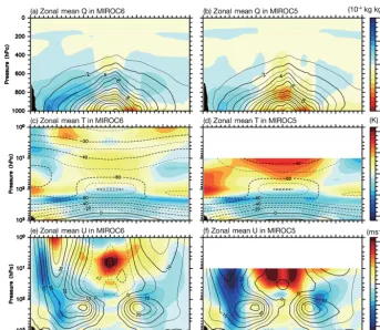
The improvement in spatial radiation patterns, especially in low-latitude OSR, is explained primarily by the im-plementation of shallow convective processes, which re-sults in a moister free troposphere in MIROC6 than in MIROC5. Figure 7a and b show zonal mean biases in annual mean specific humidity with respect to the Eu-ropean Centre for Medium-Range Weather Forecasts
Figure 5.Annual mean moistening rate associated with(a)deep convection and(b)shallow convection in MIROC6 at the 850 hPa pressure level.
model representation of precipitation in MIROC6 is not nec-essarily alleviated other than the western tropical Pacific. For example, the overestimate of wintertime precipitation over the Indian Ocean and the midlatitude North Pacific is worse in MIROC6 than in MIROC5.
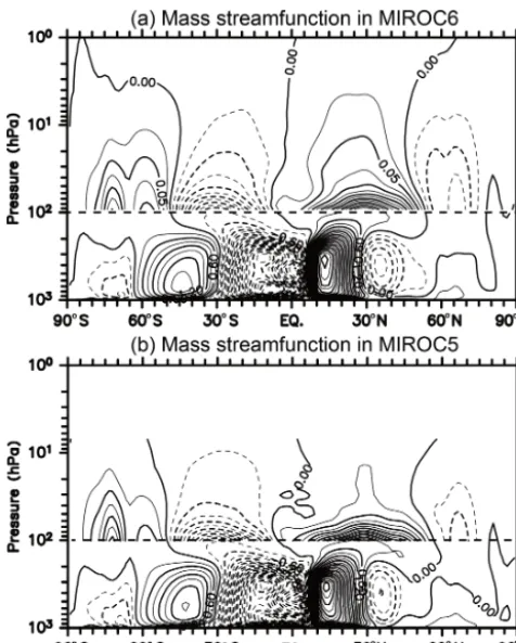
Zonal mean biases in annual mean air temperature and zonal wind velocity are also better represented in MIROC6 than in MIROC5 (Figs. 7c-f). The upper stratospheric warm bias at 50◦S–50◦N in MIROC5 is significantly reduced in MIROC6. The model top of MIROC6 is located at the 0.004 hPa pressure level and there are 42 vertical layers above the 50 hPa pressure level, while the model top of MIROC5 is placed at the 3 hPa pressure level. As a re-sult, there are significant differences in stratospheric circu-lation between the models. As shown in the annual mean mass streamfunction calculated using zonal mean merid-ional winds (Fig. 9), an upward wind continuing from the low-latitude troposphere to the stratosphere is stronger in MIROC6 than in MIROC5. An increased upward advection of the temperature minimum around the tropopause at 30◦S– 30◦N may lead to a reduction of warm temperature bias in the stratosphere, which is significant in MIROC5. Corre-spondingly, the stratospheric westerly bias at low latitudes of MIROC5 is also considerably alleviated in MIROC6. Note that the atmospheric O3concentration data used in MIROC5 are different from those in MIROC6, and the concentration in the stratosphere is higher than the data used in MIROC6. About 25 % of the abovementioned reduction in the strato-spheric warm biases is explained by the smaller absorption of shortwave radiation by O3. Note that the zonal mean
tem-perature bias in Fig. 7c is smaller when the climatological mean temperature from 1980 to 2009 in a historical simula-tion is evaluated against observasimula-tions because of the known stratospheric cooling with increased greenhouse gases and reduced O3concentrations.
The zonal means of the air temperature and zonal wind in MIROC6 are also better simulated in the middle and high latitudes. A pair of easterly and westerly biases in MIROC5, which is in the troposphere of the Northern Hemisphere, is associated with a weaker midlatitude westerly jet and its southward shift with respect to observations. The pair of biases is reduced in MIROC6, thereby suggesting that a strengthening and northward shift of the westerly jet oc-cur in MIROC6. Indeed, as shown in Fig. 10, the merid-ional contrast of high and low biases at the 500 hPa pres-sure level (Z500) along the wintertime westerly jet is weaker in MIROC6 than in MIROC5. The latitudes with the max-imal meridional gradient of Z500 are located further north-ward in MIROC6 than in MIROC5, especially over the North Atlantic. Correspondingly, wintertime storm track activity (STA), which is defined as an 8 d high-pass-filtered eddy meridional temperature flux at the 850 hPa pressure level, is stronger over the North Pacific and Atlantic in MIROC6 than in MIROC5 (see Fig. 11) and is accompanied by an associated increase in precipitation, especially in the North Pacific (Fig. 8c, e). In the stratosphere above the 10 hPa pressure level, the polar night jet is reasonably captured in MIROC6, although the westerly is somewhat overestimated at 30–60◦N. Also, in the Southern Hemisphere, representa-tion of the tropospheric westerly and the polar night jets is better in MIROC6 than in MIROC5, and the easterly bias centered at 60◦S in the troposphere is clearly reduced in MIROC6. Although causality is unclear, the warm air tem-perature bias above the tropopause to the south of 60◦S is smaller in MIROC6 than in MIROC5.
2738 H. Tatebe et al.: Basic evaluation of MIROC6
Figure 6. Same as Fig. 4, but for cloud cover in MIROC6(a, c, e)and MIROC5(b, d, f). Low-, middle-, and high-level cloud cover is aligned from the top to the bottom. The tops for low-, middle-, and high-level clouds are defined to exist below the 680 hPa, between the 680 and 440 hPa, and above the 440 hPa pressure levels, respectively. The unit is nondimensional. ISCCP climatology is used as observations.
50◦N (S) is stronger and extends further upward in MIROC6 than in MIROC5. This circulation seems to continue from the troposphere into the stratosphere, thereby implying that more active troposphere–stratosphere interactions associated with wave coupling exist in MIROC6. Further details will be described later, focusing on the occurrence of sudden strato-spheric warmings.
Parameterizations of SSNOWD (Liston, 2004; Nitta et al., 2014) and a wetland due to snowmelt water have been newly implemented into MIROC6 (Nitta et al., 2017). In comparison of MIROC6 with MIROC5, it can be seen that the former parameterization brings about significant im-provement in the Northern Hemisphere snow cover frac-tions from the early to the late winter (Fig. 12). Compared with observations of the Northern Hemisphere EASE-Grid 2.0 (Brodzik and Armstrong, 2013; the data are available at https://nsidc.org/data/ease/, last access: 1 January 2013), the distribution of the snow cover fractions is more realis-tic in MIROC6 than MIROC5, especially where and when the snow water equivalent is relatively small (e.g., middle and high latitudes in November, over Siberia in February). Note that no clear improvement is found in May. This is be-cause the newly implemented SSNOWD represents hystere-sis in the relationship between snow water equivalent and
snow cover fraction in both the accumulation and ablation seasons. MIROC6 underestimates the snow cover fraction in the partially snow-covered regions and overestimates it on the Tibetan Plateau and in some parts of China. We note that meteorological (e.g., precipitation or temperature) phenom-ena might affect these biases, but further investigation will be necessary to identify their causes. Nevertheless, in spite of those discrepancies, it can be said that the seasonal changes in the snow cover fraction are better simulated in MIROC6 than in MIROC5 (Fig. 12j).
3.1.2 Ocean
for-Figure 7.Annual and zonal mean specific humidity(a, b), temperature(c, d), and zonal wind(e, f)in MIROC6(a, c, e)and MIROC5(b, d, f). Colors indicate errors with respect to observations (ERA-I) and contours denote values in each model.
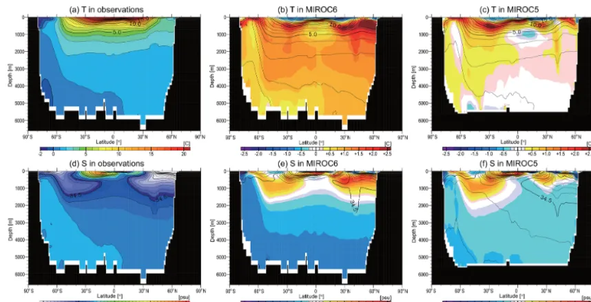
mation is also found at the northern high latitudes of the At-lantic sector (Figs. 13a–c). By horizontal advection of the warm temperature biases associated with the Pacific and At-lantic MOC, the model temperatures in deep layers apart from polar regions are also warmer than in observations. The warm potential temperature bias in the deep layer is worse in MIROC6 than in MIROC5 in both the Atlantic and Pacific sectors, and the warm bias influences the subsurface and the intermediate layers above the 3000 m depth, which might be attributed to the excess ocean heat uptake and longer inte-gration time in MIROC6 than in MIROC5 (the spin-up dura-tion of MIROC6 is 2000 years and that of MIROC5 is about 1000 years). Also, the low-salinity bias below the 2000 m depth is worse in MIROC6 than in MIROC5, especially in the Pacific sector (Fig. 14e, f). This worsening can be ex-plained by the excess supply of the freshwater in the South-ern Ocean and weaker northward intrusion of the less saline water in MIROC6.
In the Arctic Ocean, the halocline above the upper 500 m of depth is sharper and more realistic in MIROC6 than in MIROC5 and the high-salinity bias below the 500 m depth in MIROC5 is alleviated in MIROC6 (Fig. 13e, f) because, as described in Sect. 2.3, there are many more vertical levels in the surface and subsurface layers of MIROC6. In addi-tion, vertical diffusivity in the Arctic Ocean is set to smaller
values in MIROC6 than in MIROC5, and the turbulent ki-netic energy input induced by surface wave breaking, as a function of the sea ice concentration in each grid cell, is reduced in MIROC6, as shown in Komuro (2014). In the North Pacific, the southward intrusion of North Pacific In-termediate Water (NPIW) around the 1000 m depth retreats northward in MIROC6. Strong tide-induced vertical mixing of seawater is observed along the Kuril Islands (e.g., Kat-sumata et al., 2004). The locally enhanced tide-induced mix-ing is known to reinforce the southward intrusion of the Oy-ashio and associated water mass transport from the subarctic to subtropical North Pacific and to feed the salinity minimum of NPIW (Nakamura et al., 2004; Tatebe and Yasuda, 2004). Hence, NPIW reproducibility is better in MIROC5, in which enhanced tidal mixing is considered, than in MIROC6. Be-cause we encountered significant uncertainty in implement-ing the tidal miximplement-ing, we decided to stop implementimplement-ing it in the development phase of MIROC6 at the expense of NPIW reproducibility.
2740 H. Tatebe et al.: Basic evaluation of MIROC6
Figure 8.Precipitation in boreal winter (December–February;a, c, e) and summer (June–August;b, d, f) in observations (a, b; GPCP), MIROC6(c, d), and MIROC5(e, f). Areas with precipitation less than 3 mm d−1are not colored.
thermocline. The eastward speed of the Equatorial Under-current in MIROC6 is over 80 cm s−1, and is closer to the products of Simple Ocean Data Assimilation (SODA; Carton and Giese, 2008; the data are available at http://www.soda. umd.edu/, last access: 15 February 2019) than in MIROC5. These improvements are mainly attributed to the higher verti-cal resolution of MIROC6 in the surface and subsurface lay-ers. However, the thermocline depths in the western tropi-cal Pacific are still larger in the models than in observations and are attributed to the stronger trade winds in the models. When both MIROC6 and MIROC5 are executed as stand-alone AGCMs with the prescribed SST obtained from ob-servations, the an overestimate of the equatorial trade winds also appears due to overestimate of the upward winds over the maritime continent associated with deep cumulus con-vection and the resultant strengthening of the Walker circu-lation over the equatorial Pacific. Better parameterizing deep cumulus convection in the models would be required for a better representation of the equatorial trade winds and thus oceanic states.
Figure 16 displays annual mean Atlantic and Pacific MOC. In the Atlantic, two deep circulation cells associated with North Atlantic Deep Water (NADW; upper cell) and Antarc-tic Bottom Water (AABW; lower cell) are found in both of the models. NADW transport across 26.5◦N is 17.2 (17.6) Sv (1 Sv=106m3s−1) in MIROC6 (MIROC5). These values are consistent with the observational estimate of 17.2 Sv
(McCarthy et al., 2015). RMS amplitudes of NADW trans-port are about 0.9 Sv in MIROC6 and 1.1 Sv in MIROC5 on longer than interannual timescales. These are smaller than the observed amplitude of 1.6 Sv in 2005–2014. Because observations include the weakening trend of the Atlantic MOC due to global warming, they can be larger than the model variability under preindustrial conditions. In the Pa-cific Ocean, both the models have the deep circulation asso-ciated with Circumpolar Deep Water (CDW), but the north-ward transport of CDW across 10◦S is 8.6 Sv in MIROC6, which is slightly larger than 7.5 Sv in MIROC5. Although these model values are somewhat smaller than observations, they are within the uncertainty range of observations (Talley et al., 2003; Kawabe and Fujio, 2010).
Figure 9.Annual mean mass streamfunctions in(a)MIROC6 and
(b) MIROC5. Contour interval is 0.3(0.025)×1010kg s−1below (above) the 100 hPa pressure level. Negative values are denoted by dashed contours, and the horizontal dashed lines indicate the 100 hPa pressure level.
Lawrence, even though the sea ice area in the former region is better simulated in MIROC6 than in MIROC5. Meanwhile, the eastward retreat of the sea ice in the Barents Sea is better represented in MIROC6 than in MIROC5. The overestimates in September in the models are due to the model climatol-ogy being defined under preindustrial conditions, while ob-servations are taken in present-day conditions of 1980–2009 when a rapid decreasing trend of summertime sea ice area (including a few events of drastic decreases) is ongoing (e.g., Comiso et al., 2008). Note that the model September sea ice area in 1980–2009 from historical simulations is smaller than the observations, and the sea ice area does not show a dras-tic year-to-year sea ice decrease with comparable amplitude with observations. The underestimate of the mean Septem-ber sea ice area in MIROC6 might be attributed to slightly more rapid warming of the Arctic climate in MIROC6 than in observations. On the other hand, the modeled sea ice ar-eas in the Southern Ocean are unrealistically smaller than in observations. Southern Hemisphere sea ice areas in March (September) are 0.1 (3.4), 0.2 (5.2), and 5.0 (18.4) million square kilometers in MIROC6, MIROC5, and observations, respectively. Since there are no significant differences
be-tween the two models, the spatial maps for the sea ice area in the Southern Hemisphere are omitted.
Figure 18 shows the global maps of annual mean sea level height relative to the geoid. The absolute dynamic height values provided by Archiving, Validation, and Interpretation of Satellite Oceanographic (AVISO; Rio et al., 2014) data are used as observed sea level height (the data are avail-able at https://www.aviso.altimetry.fr/en/home.html, last ac-cess: 20 June 2019). Overall, oceanic gyre structures in the two models are consistent with observations. Although rep-resentation of the gyres in MIROC6 remains generally the same as in MIROC5, there are a few improvements in the North Pacific and the North Atlantic. The midlatitude west-erly in MIROC6 is stronger and is shifted further northward than in MIROC5 (Fig. 10), which results in the strengthen-ing of the subtropical gyres, northward shifts of the west-ern boundary currents, and their extensions. In particular, the current speed of the Gulf Stream and the North Atlantic Current is faster in MIROC6 than in MIROC5, and the con-tours emanating from the North Atlantic reach the Barents Sea in MIROC6. A corresponding increase in warm water transport from the North Atlantic to the Barents Sea leads to sea ice melting and an eastward retreat of the wintertime sea ice there in MIROC6 (Fig. 17a–c). An improvement in MIROC6 is also found in the Subtropical Countercurrent (STCC) in the North Pacific along 20◦N. As reported in Kubokawa and Inui (1999), the low-potential-vorticity wa-ter associated with a winwa-tertime mixed layer deepening in the western boundary current region is transported southward in the subsurface layer, and it pushes up isopycnal surfaces around 25◦N. Thus, the eastward-flowing STCC is induced around 25◦N. Although both of the models show the win-tertime mixed layer deepening, the ocean stratification along 160◦E is weaker in MIROC6 than in MIROC5 (not shown). This suggests that the isopycnal advection of low-potential-vorticity water in MIROC6 is more realistic than in MIROC5.
re-2742 H. Tatebe et al.: Basic evaluation of MIROC6
Figure 10.Same as Fig. 4, but for the wintertime 500 hPa pressure level in MIROC6(a, c)and MIROC5(b, d). Maps for boreal and austral winter are shown in(a, b)and(c, d), respectively. ERA-I is used as observations.
Figure 11.Wintertime storm track activity (STA) in observations(a, d), MIROC6(b, e), and MIROC5(c, f). STA is defined as 8 d high-pass-filtered eddy meridional temperature flux at the 850 hPa pressure level. Maps for boreal and austral winter are shown in(a–c)and(d–f), respectively. ERA-I is used as observations.
semble those in MIROC5, there are several improvements. For example, cold SAT bias in MIROC5 extending from the Barents Sea to Eurasia is significantly smaller in MIROC6, possibly owing to the increase in warm water transport by the North Atlantic Current and the resultant eastward retreat of the sea ice in the Barents Sea (Figs. 17 and 18). Warm SAT and SST biases along the west coast of North America are smaller in MIROC6 than in MIROC5. The reason is that an increase in southeastward Ekman transport in the eastern subarctic North Pacific due to the strengthening of the mid-latitude westerly jet (Fig. 10) and the Aleutian low tend to cancel out the relatively warm water supply from the subtrop-ics to the subarctic region by the surface geostrophic current. Although it is not clear from Fig. 19, the SAT and SST in the subtropical North Pacific around 20◦N are warmer by 2 K in MIROC6 than in MIROC5. Also in the Atlantic, the SAT in the western tropics is warmer in MIROC6. These warmer surface temperatures in MIROC6 indicate a reduction of the cold SAT and SST biases that can be alleviated by an increase in the downward OSR in MIROC6 due to the implementation of a shallow convective parameterization (Fig. 4) and by an increase in eastward transport of the warm pool temperature associated with the stronger STCC in MIROC6 (Fig. 18).
On the other hand, the warm SAT and SST biases in the Southern Ocean and the warm SAT bias in the Middle East and the Mediterranean are worse in MIROC6 than in MIROC5. Consequently, the RMS error in SAT is larger in
MIROC6 (2.4 K) than in MIROC5 (2.2 K). The former is es-sentially due to the underestimate of mid-level cloud cover, excess downward OSR, and the resultant underestimate of the sea ice in the Southern Ocean. Such a bias commonly occurs in many climate models and is normally attributed to errors in cloud radiative processes (e.g., Bodas-Salcedo et al., 2012; Williams et al., 2013). In addition, poor represen-tations of mixed layer depths and open-ocean deep convec-tion due to the lack of mesoscale processes in the Antarctic Circumpolar Current are causes of the warm bias (Olbers et al., 2004; Downes and Hogg, 2013). The latter warm bias, seen in the Middle East around the Mediterranean, can be explained by a tendency to underestimate the radiative forc-ing of aerosol–radiation interactions due to an underestimate of dust emissions from the Sahara in MIROC6 (not shown).
3.2 Internal climate variations
3.2.1 Madden–Julian oscillation and East Asian monsoon
Figure 12.Snow cover fractions for observations(a, d, g), MIROC6(b, e, h), and MIROC5(c, f, j). Maps in November, February, and May are aligned from the left to the right. The unit is nondimensional. Areas where snow cover fractions are less than 0.01 are masked. “Ave” and “corr” in the panels indicate spatial averages and correlation coefficients between observations and models over the land surface in the Northern Hemisphere, respectively. Time series in(j)shows the temporal rate of change of the monthly spatial averages. The snow cover dataset of the Northern Hemisphere EASE-Grid 2.0 is used as observations.
Figure 13.Annual mean potential temperature (a, b, c; unit is◦C) and salinity (d, e, f; psu) in the Atlantic sector for observations(a, d), MIROC6(b, e), and MIROC5(c, f). Colors indicate errors with respect to observations (ProjD) and contours denote model values in(b, e)
and(c, f).
OLR are calculated following Wheeler and Kiladis (1999) and are shown in Fig. 20. The daily mean OLR data de-rived from the Advanced Very High Resolution Radiome-ter (AVHRR) of the National Oceanic and Atmospheric Ad-ministration (NOAA) satellites (Liebmann and Smith, 1996; the data are available at https://www.esrl.noaa.gov/psd/data/
gridded/data.interp_OLR.html, last access: 8 April 2019) are used for observational references. The signals corresponding to the Madden–Julian oscillation (MJO), equatorial Kelvin (EK), equatorial Rossby (ER), eastward inertia–gravity (n=
2744 H. Tatebe et al.: Basic evaluation of MIROC6
Figure 14.Same as Fig. 13, but for the Pacific sector.
and eastward inertia–gravity (n=0 EIG) waves in the an-tisymmetric component stand out from the background spec-tra in observations. MIROC5 qualitatively reproduces these spectral maxima of the symmetric MJO, EK, and ER quali-tatively, while the amplitudes of the MJO and the EK are un-derestimated. These underestimates are partially mitigated in MIROC6. The power summed over the eastward wavenum-bers 1–3 and periods of 30–60 d corresponding to the MJO is 20 % larger in MIROC6 than in MIROC5. Furthermore, some additional analyses indicate that many aspects of the MJO, including its eastward propagation over the western tropical Pacific, are improved in MIROC6. Those improve-ments are primarily associated with the implementation of the shallow convective scheme that moistens the lower tro-posphere. The results of these additional analyses, along with some sensitivity experiments, are described in a separate pa-per (Hirota et al., 2018). The EIG and WIG in the symmetric component and the MRG and the EIG in the antisymmetric component are missing in both MIROC6 and MIROC5.
Figure 21 shows the June–August (JJA) climatology of precipitation and circulation in East Asia. As shown in ob-servations (ERA-I; Fig. 21a), the East Asian summer mon-soon (EASM) is characterized by the monmon-soon low over the warmer Eurasian continent and the subtropical high over the colder Pacific Ocean (e.g., Ninomiya and Akiyama, 1992). The southwesterly between these pressure systems transports moist air to the midlatitudes, forming a rainband calledBaiu
in Japanese. The general circulation pattern of the EASM and the rainband are well simulated in both MIROC6 and MIROC5. It should be noted that one of major deficiencies in MIROC5, the underestimate of the precipitation around the Philippines, has been largely alleviated in MIROC6. This improvement is, again, associated with the moistening of
the lower troposphere by shallow convective processes. In-terannual EASM variabilities are examined using an empir-ical orthogonal function (EOF) analysis of vorticity at the 850 hPa pressure level over [100–150◦E, 0–60◦N] following Kosaka and Nakamura (2010). The regressions of precipi-tation and 850hPa vorticity with respect to the time series of the first mode (EOF1) are shown in Fig. 21. In observa-tions, precipitation and vorticity anomalies show a tripolar pattern with centers located around the Philippines, Japan, and the Sea of Okhotsk (Hirota and Takahashi, 2012). The anomalies around the Philippines and Japan correspond to the so-called Pacific–Japan pattern (Nitta et al., 1987). The southwest–northeast orientation of the wave-like anomalies is better simulated in MIROC6 than in MIROC5.
Figure 15. Annual mean climatology of potential temperature (◦C; colors) and zonal current speed (cm s−1; contours) along the Equator (1◦S–1◦N) in (a)observations (ProjD and SODA),
(b)MIROC6, and(c)MIROC5.
previous studies (Fig. 22d; e.g., Nakamura, 1992). This rela-tionship between the circulation and the STA can be found in MIROC6 but not in MIROC5 (Fig. 22e, f). The explained variance of the EOF1 is 46.0 % in observations, 37.1 % in MIROC5, and 47.1 % in MIROC6, suggesting that the am-plitude of this variability in MIROC6 is consistent with ob-servations.
3.2.2 Stratospheric circulation
A few of the major changes in the model setting from MIROC5 to MIROC6 are higher vertical resolution and higher model-top altitude in MIROC6, namely the represen-tation of the stratospheric circulation. Here, we examine the
representation of the quasi-biennial oscillations (QBOs) in MIROC6. Figure 23 shows the time–height cross sections of the monthly mean, zonal-mean zonal wind over the Equator for observations (ERA-I) and MIROC6. In this figure, an ob-vious QBO with a mean period of approximately 22 months can be seen in MIROC6. The mean period is slightly shorter than that of∼28 months in observations, and the simulated QBO period varies slightly from cycle to cycle. The maxi-mum speed of the easterly at the 20 hPa pressure level is ap-proximately−25 m s−1in MIROC6 and that of the westerly is 15 m s−1. On the other hand, the observed maximum wind speeds are−35 m s−1 for the easterly and 20 m s−1for the westerly. The simulated QBO has a somewhat weaker ampli-tude in MIROC6 than observations but the same east–west phase asymmetry. The QBO in MIROC6 shifts upward com-pared with that in observations, and the simulated amplitude is larger above the 5 hPa pressure level and smaller in the lower stratosphere. The simulated downward propagation of the westerly shear zones of zonal wind (∂u
∂z >0, where
zis the altitude) is faster than the downward propagation of easterly shear zones (∂u
∂z ) <0, which agrees with obser-vations. The QBOs in MIROC6 are qualitatively similar to that represented in the MIROC ESM, which is an Earth sys-tem model with a similar vertical resolution that participated in CMIP5 (Watanabe et al., 2011). Note that nothing resem-bling a realistic QBO was simulated in the previous low-top version of MIROC5, which only has a few vertical layers in the stratosphere.
Recently, Yoo and Son (2016) found that the observed MJO amplitude in the boreal winter is stronger than normal during the QBO easterly phase at the 50 hPa pressure level. They also showed that the QBO exerted greater influence on the MJO than did ENSO. Marshall et al. (2016) pointed out the improvement in forecast skill during the easterly phase of the QBO and indicated that the QBO could be a potential source of the MJO predictability. MIROC6 successfully sim-ulates both the MJO and QBO in a way consistent with ob-servations, as mentioned above, but correlations between the QBO and MJO are insignificant. One possible reason is the smaller amplitude of the simulated QBO in the lowermost stratosphere. The QBO contribution to tropical temperature variation at the 100 hPa pressure level is∼0.1 K in MIROC6, which is much smaller than the observed value of∼0.5 K (Randel et al., 2000). The simulated QBO has little effect on static stability and vertical wind shear in the tropical upper troposphere.
Hemi-2746 H. Tatebe et al.: Basic evaluation of MIROC6
Figure 16.Annual mean meridional overturning circulation in the Atlantic(a, b)and the Indo-Pacific sectors(c, d)in MIROC6(a, c)and MIROC5(b, d). The unit is the sverdrup (Sv;≡106m3s−1).
Figure 17.Northern Hemisphere sea ice concentrations in March(a, b, c)and September(d, e, f)for observations(a, d), MIROC6b, e), and MIROC5(c, f). The unit is nondimensional. Satellite-based sea ice concentration data of the SSM/I are used as observations.
sphere in observations (Fig. 24a), which correspond to QBO and polar vortex variability. This feature is well captured in MIROC6 (Fig. 24b), while there are too-small variations in MIROC5 where the stratosphere cannot be well resolved (Fig. 24c). The better representation of polar vortex
con-Figure 18.Annual mean sea level height relative to the geoid in
(a)observations,(b)MIROC6, and(c)MIROC5. Contour interval is 20 cm. Negative values are denoted by dashed lines. Note that loading due to sea ice and accumulated snow on sea ice are removed from the model sea level height and that the global mean value is eliminated.
sistent with previous modeling studies that reported the im-portance of the well-resolved stratosphere for better simula-tion of stratospheric variability (e.g., Cagnazzo and Manzini, 2009; Charlton-Perez et al., 2013; Osprey et al., 2013). In December–January, however, MIROC6 still underestimates the frequency of SSW events, which is a common bias in other high-top climate models (e.g., Inatsu et al., 2007; Charlton-Perez et al., 2013; Osprey et al., 2013). It is conjec-tured that the less frequent SSW in December–January could be attributed to less frequent stationary wave breaking due to an overestimate of the climatological zonal wind speed of the polar night jet in MIROC6 (Fig. 24d and e).
The inclusion of a well-resolved stratosphere in MIROC6 is also considered to be important for improvement in the
representation of stratosphere–troposphere coupling. In or-der to evaluate this, we examine the time development of the northern annular modes (NAMs) associated with strongly weakened polar vortex events in the stratosphere. The NAM indices are defined by the first EOF mode of the zonal mean year-round daily geopotential height anomalies over the Northern Hemisphere and are computed separately at each pressure level (Baldwin and Thompson, 2009). The height anomalies are first filtered by a 10 d low-pass filter to remove transient eddies. Figure 25 shows the composite of the time development of the NAM index for weak polar vor-tex events. The events are determined by the dates on which the 10 hPa NAM index exceeded−3.0 standard deviations (Baldwin and Dunkerton, 2001). Note that the NAM index is multiplied by the square root of the eigenvalue in each level before the composite, that is, the composite having the geopotential height dimension. The weak polar vortex sig-nal in the stratosphere propagates downward to the surface and persists for approximately 60 d in the lower stratosphere and upper troposphere. These observational features are well represented in MIROC6 (Fig. 25a, b). Although MIROC5 has also captured downward-propagating signals, its magni-tude is approximately half in the stratosphere, and its per-sistency is weak in the lower stratosphere and upper tro-posphere. Therefore, these results strongly indicate that the inclusion of a well-resolved stratosphere in a model is im-portant for representing not only stratospheric variability, but also stratosphere–troposphere coupling.
3.2.3 El Niño–Southern Oscillation and Indian Ocean Dipole mode
2748 H. Tatebe et al.: Basic evaluation of MIROC6
Figure 19. Same as Fig. 4, but for annual mean SAT(a, b)and SST(c, d). ERA-I for the SAT and the ProjD for the SST are used as observations.