BIBECHANA
A Multidisciplinary Journal of Science, Technology and Mathematics
ISSN 2091-0762 (Print), 2382-5340 (0nline)
Journal homepage: http://nepjol.info/index.php/BIBECHANA
Publisher: Research Council of Science and Technology, Biratnagar, Nepal
Correlation of solar wind velocity with different parameters
during geomagnetic disturbances
Sujan Dhakal1, Binod Adhikari1,2*, Kiran Pudasainee2, Naryan Prasad Chapagain2,3 Drabindra
Pandit1,2,3 Subodh Dahal4, Bikash Shrestha1, Bhawani Sapkota4, Daya Nidhi Chhatkuli5
1St. Xavier’s College, Maitighar, Kathmandu, Nepal
2Patan Multiple Campus, Patandhoka, Lalitpur, Nepal
3Central Department of Physics, Tribhuvan University, Kirtipur, Kathmandu, Nepal
4Department of Physics, Himalayan College of Geomatic Engineering and LRM, Kathmandu
5Department of Physics, Tri-Chandra Multiple Campus, Kathmandu, Nepal
*E-mail: [email protected]
Article history: Received 29 April, 2018; Accepted 04 November, 2018
DOI: http://dx.doi.org/10.3126/bibechana.v16i0.21575
This work is licensed under the Creative Commons CC BY-NC License. https://creativecommons.org/licenses/by-nc/4.0/
Abstract
We have studied the solar wind velocity and it’s relation with solar wind pressure, southward component of IMF-Bz, solar wind temperature (Tsw), solar wind density (Nsw) and geomagnetic indices during different geomagnetic disturbances. During disturbed days, there is a fluctuation of energy and plasma inside the magnetosphere, which changes the parameters like pressure, velocity, IMF-Bz, SYM-H and AE indices. The solar wind velocity shows very remarkable relationship with pressure. There is weak connection of solar wind pressure with IMF-Bz, although it is more geo-effective.
Keywords: Geomagnetic storm; solar wind velocity; cross-correlation analysis.
1. Introduction
turmoil in geomagnetic activity resulting into geomagnetic storms, substorms as well as HILDCAAs (high intensity long duration continuous auroral activities) [6,7]. Generally, the most intense geomagnetic storms are due to CMEs whereas CIRs cause less intense geomagnetic storms [8]. The intensity of the geomagnetic storm depends upon the solar wind structures [9]. A typical geomagnetic storm is caused by a solar wind shock wave and/or cloud of magnetic field that interacts with the Earth’s magnetic field [3]. Both interactions increase plasma movement through the magnetosphere that increase an electric current in the magnetosphere. The impact of different solar phenomenon is measured by solar wind parameters and geomagnetic indices. Geomagnetic storm cause changes in geomagnetic indices such as Disturbance storm time (Dst), Kp, AE etc. Geomagnetic indices are ground based measurements that are collected to quantify the state of the magnetosphere and it shows how the Earth reacts to given wind structure. These indices perturbation give the idea of the Earth’s magnetosphere which is continuously affected by the solar wind flowing from the sun’s corona [2, 10, 11]. Geomagnetic indices are the measure of the geomagnetic activity which plays the significance role in describing the space weather. Space weather refers to highly vulnerable conditions in the near earth space environment. The geomagnetic indices are used to quantify the ability and geo-effectiveness of interplanetary solar wind structure to cause geomagnetic storms [5,6]. The increase in the solar wind pressure initially can compress the magnetosphere [11].
2. Dataset and Methodology
The data for this study have extracted the OMNI (Operating Mission as Nodes on the Internet) wave page and downloaded from the official website of NASA https://omniweb.gsfc.nasa.gov/data set for solar wind measurements.
Cross-correlation
Cross-correlation is simply a measure of statistical relationships involving two or more variables as a function of time lags applied to one of them. One can simply understand the cross correlation as a measure of similarities of two different time series function, one relative to the other. It is also known as sliding dot product or sliding inner product. Its value ranges from -1 to 1 and with the highest degree of cross correlation its value is close to 1. It is the standard method to estimate the degree to which two different series are correlated.
3. Result and Discussion
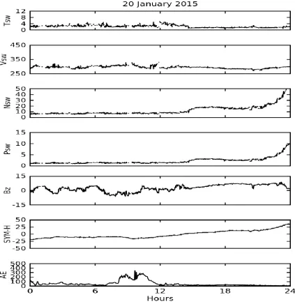
In this section, we are dealing with cross correlation of solar wind velocity with component of IMF (Bz) and geomagnetic indices for four different geomagnetic disturbance on different period. Mainly correlation between Vsw with solar wind parameter Psw, SYM-H and AE are analyzed. The brief discussion of the event using solar wind parameter and interplanetary parameters are discussed below. Event 1: January 20, 2015
The variation of Sq-H is characterized maximum around the daytime (07:00-17:00LT) and the minimum values during pre-sunrise hours between 05:00 and 06:00LT. It is clear that before the sunrise, conductivities are low due to absence of solar thermal heating. Due to lack of solar thermal heating causes the ionosphere conductivities to be the weakest pre-sunrise hours over all the day throughout the year. During a geomagnetic disturbance, there is an energy input inside the magnetosphere which changes atmospheric parameters. But during quiet periods, the disturbances measurements on the ground are less significant.
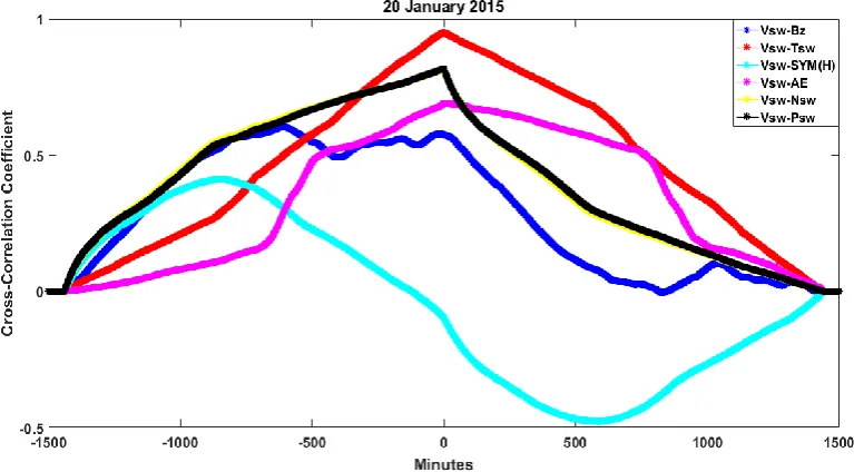
Figure 2 shows the cross-correlation of Vsw with solar parameters and geomagnetic indices during 20th January 2015. The horizontal axis represents the scale in minutes and the vertical axis represents the cross-correlation coefficient. The red curve shows the correlation between Vsw and Tsw is highly positive with coefficient around 1. The sky-blue curve shows correlation between Vsw-SYM-H is moderate and sometime crosses the zero points and reaches a negative value around -0.5. The Psw-Bz (blue curve) shows positive correlation with correlation coefficient around 0.6 at time lag -800 minutes. Similarly, the Vsw-AE (pink curve) and Vsw-Nsw (yellow curve) shows positive correlation with correlation coefficient around +0.7 and +0.8 respectively. The Vsw-Psw (black curve) shows similar nature as yellow curve with correlation coefficient +0.8. Here moderately and less correlated line seems to be more irregular and fluctuating than the highly correlated ones.
Fig. 2: Cross-correlation of solar wind velocity with southward component of interplanetary magnetic field (Bz), solar wind temperature (Tsw), SYM (H), AE solar wind density (Nsw), and solar wind pressure respectively during 20th January 2015.
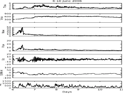
Event 2: 6-10 June 2006
the recovery phase is longer in the year 1974.The Dst recoveries are associated with high AE values. The main reason for this is high fluctuation in interplanetary Bz in the high velocity stream. With every instant of southward field turnings, there is an increase in AE and decrease in Dst. The southward turnings cause magnetic reconnection and plasma injections into the night side magnetosphere. There is slight decrease in Dst at each of these injections. These periods of continuous substorm activity are defined as HILDCAA. The main cause of the interplanetary Bz fluctuations is given by Belcher and Davis (1971). They have demonstrated that Alfven waves are propagating away from the sun which are present in the high-speed streams leads to the Bz fluctuations within the CIRs leading to the irregular shaped storm main phase, and also the fluctuations that cause HILDCAAs in the storm “recovery phases”. [7] Has described the seasonal dependence of HILDCAA events to determine the solar cycle. Their study clarifies that the occurrence of HILDCAA events during the different phases of the solar cycle. That paper also discussed the interplanetary Alfven waves by indicating high IMF BZ variance and normalized variance of the HILDCAA events. [12,13] studied the solar wind energy during HILDCAA in his PhD thesis to described the electrodynamical process caused by the solar wind magnetosphere coupling for HILDCAA events (high intensity, long duration continuous AE activity) [12,14]. He has also described the effect of HILDCAA event on geomagnetic status and its consequence on Earth’s environment by analysing the coupling mechanism between the solar wind and magnetosphere.
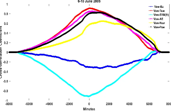
Figure 4 shows the cross-correlation of Vsw with solar parameters and geomagnetic indices during 6-10 June 2006. The horizontal axis represents the scale in minutes and the vertical axis represents the cross-correlation coefficient. In this figure, the sky-blue curve shows negative cross-correlation coefficient of around -0.90 between SYM-H-Vsw with a time lag around 10 minutes and it does not show any positive correlation during this event. The negative correlation signifies that if the value of Vsw decreases with time then SYM-H increases with increasing time and vice-versa. This means they have a negative relationship with each other. Similarly, red curve shows positive correlation between Vsw-Psw with high correlation coefficient of about 0.9. The Vsw-AE pink curve has a good positive cross-correlation with correlation coefficient of about 0.78 at zero-time lag. Similarly, the Vsw-Psw black curve and Vsw –Nsw yellow curve also shows good positive cross-correlation with correlation coefficient of about 0.76 and 0.60 at 0-time lag respectively. Blue curve ( Vsw-Bz) shows negative correlation with correlation coefficient of about -0.3 at 0 minutes time lag.
Fig. 4: Cross-correlation of solar wind velocity with southward component of interplanetary magnetic field (Bz), solar wind temperature (Tsw), SYM(H), AE solar wind density (Nsw), and solar wind pressure respectively during (6-10) June 2006.
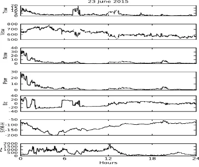
Event 3: 23 June 2015
due to the direct dependence of the geomagnetic storm with south-north component of magnetic field Bz. According to Gonzalez et al. (1992), the intense interplanetary field can be thought of a high- speed stream, the intrinsic ejecta (called driver gas fields) and the shocked and compressed fields and plasma due to the collision of the high-speed stream with the slower solar wind preceding it. The greater the relative velocity, the stronger is the shock and the field compression, had investigated the effect of solar wind dynamic pressure Psw, and preconditioning over 80 large magnetic storms (Dst<-100nT) which was occurring during solar cycle 23, and found that in the main phase of a storm, when there is a large enhancement of the dynamic pressure, there is always an increase in the Dst peak value during the storm main phase, the weak Psw verses Vsw relationship was connected to the ring current energy losses which may be originated from different sources. The solar wind dynamic pressure has a strong relationship with the southward IMF Bz during the main phase of a storm, typically when the plasma flow speed value is very large, exceeding the 650 km/s value, and the Dst<-100nT.
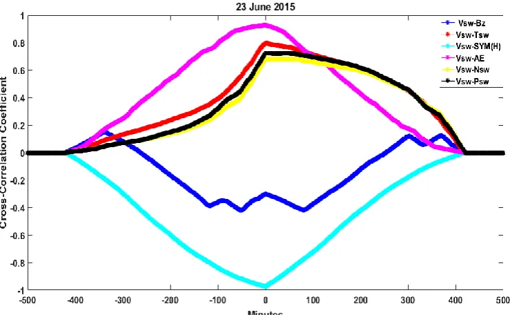
Figure 6 represents the cross-correlation of Vsw with solar parameters and geomagnetic indices during 23 June 2015. Here the horizontal axis represents the scale in minutes and the vertical axis represents the cross-correlation coefficient. The pink curve shows the correlation between AE and Vsw. This curve represents strong positive cross-correlation coefficient of about 0.8 at lag zero. The sky-blue curve shows good correlation between Vsw-SYM-H with cross-correlation coefficient of around -1 at lag of zero minutes. The negative correlation signifies that if the value of Vsw decreases with time then SYM-H increases with time and vice-versa. The blue curve of Vsw-Bz represents uncorrelated. The red curve represent correlation between Vsw-Tsw and it shows good correlation with correlation coefficient of about 0.75 at lag zero. Similarly, the correlation between Vsw-Nsw and Vsw-psw are represented by yellow and black color respectively. They shows good positive cross-correlation of cross-correlation coefficient about 0.6 at zero lag.
Fig. 6: Cross-correlation of solar wind velocity with southward component of interplanetary magnetic field (Bz), solar wind temperature (Tsw), SYM(H), AE solar wind density (Nsw), and solar wind pressure respectively during 23 June 2015.
Event 4: 01 March 2011
The solar wind parameters, interplanetary magnetic field fluctuation show low values, characterizing this as moderate sub-storm. During the period of substorm the Dst and IMF Bz has peak value of – 50nT and 15.01 nT respectively whereas other parameters such as solar wind speed, and AE has maximum value. The increases in the Dst and the SYM H indices after substorm onsets are related to the depolarization. This shows that about one third of the northward equatorial magnetic field variations are associated with variations in the solar wind pressure, a second third with substorm onsets, and the final third with interplanetary magnetic field reorientations in the north-south direction. Substorms are fundamental and dynamic processes in the magnetosphere, converting captured solar wind magnetic energy into plasma energy [13,14, 15]. These substorms have been suggested to be a key driver of energetic electron enhancements in the outer radiation belts. The storage and release of energetic electron during substorms in the radiation belt leads to characteristic changes in auroral morphology and emission intensity in the polar ionosphere and high-latitude surface magnetic field [16,17, 18]. The occurrence rate of substorms is more frequent and more intense during geomagnetic storms [3]. The typical duration of substorm is about 2-4 hours. The length of growth, expansion and recovery phases vary from the short expansion of 15–20 min to a lengthy growth or recovery of a few hours [19,20,21].
Figure 8 the cross-correlation of Vsw with solar parameters and geomagnetic indices during 23 June 2015. Here the horizontal axis represents the scale in minutes and the vertical axis represents the cross-correlation coefficient. The black curve shows the correlation between Vsw and Psw. The curve shows strong positive cross-correlation coefficient of about 0.9 at lag zero. The sky-blue curve shows correlation between Vsw-SYM-H is moderate and sometime crosses the zero points. The correlation between Vsw-SYM-H is represented by pink curve shows high negative cross-correlation coefficient of around 0.8 at lag of -20 minutes. The negative correlation signifies that if the value of Vsw decreases with time then SYM-H increases with increasing time and vice-versa. The blue curve of Bz-Vsw represents there week correlation. The correlation between Bz-Vsw-Nsw (yellow curve) shows good correlation with correlation coefficient about 0.85 at lag zero. Similarly, pink curve also shows good positive cross-correlation between Vsw-AE with correlation coefficient of about 0.8 at zero lag. The correlation between Vsw and Tsw is positive with correlation coefficient of about 0.80 at lag zero.
Fig. 8: Cross-correlation of solar wind velocity with southward component of interplanetary magnetic field (Bz), solar wind temperature (Tsw), SYM(H), AE solar wind density (Nsw), and solar wind pressure respectively 1st march 2011.
4. Conclusion
In this study, we have studied correlation of solar wind velocity with different solar and interplanetary indices during four different geomagnetic disturbances. This study shows the major sources of the geomagnetic disturbance are recognized to be CME, CIR, etc. The interaction of solar wind component with Earth’s magnetosphere can cause geomagnetic storms, substorms, supersubstorms, HILDCAA, etc. The conclusions are summarized as the follows:
• The solar wind velocity shows positive correlation with pressure and negative correlation with SYM/H in every event.
• There is weak connection of solar wind pressure with IMF-Bz, although it is more geo-effective.
• The strong correlation between solar wind pressure and velocity during storms initial phase was linked to the accelerated ring current build-up.
Acknowledgements
The data sets for this study were downloaded from NASA website
(http://omniweb.gsfc.nasa.gov/ow_min.html. and www.cosmic.ucar.edu/). We would like to thank NASA.
References
[1] B.T. Tsurutani, W.D. Gonzalez, F. Tang, S. Akasofu, and E. Smith, Origin of interplanetary southward magnetic fields response for major magnetic storms near solar maximum (1978-1979), J. Geophys. Res. A8 (1988) 8519 - 8531. doi.org/10.1029/JA093iA08p08519.
[2] J. T. Gosling, Coronal mass ejections and magnetic flux ropes in interplanetary space, Geophys. Monog. 58 (1990) 343–364. doi.org/10.1029/GM058p0343.
[3] W. D. Gonzalez, J. A. Joselyn, Y. Kamide, H. W. Kroehl, G. Rostoker, B. T. Tsurutani, V. M. Vasyliunas, What is a Geomagnetic Storm? J. Geophys. Res, 99 ((1994) 5771–5792. doi.org/10.1029/93JA02867.
[4] S.I. Akasofu, Solar-wind disturbances and the solar wind-magnetosphere energy coupling function, Space Sci. Rev. 34 (1983) 173-183. doi.org/10.1007/BF00194625.
[5] Elliott, H. A., J.‐M. Jahn, and D. J. McComas (2013), The Kp index and solar wind speed relationship: Insights for improving space weather forecasts, Space Weather, 11(2013)339–349 doi.org/10.1002/swe.20053.
[6] B. Adhakari, HILDCAA-Related Effects Recorded in Middle-Low Latitude Magnetometers. PhD Doctoral Dissertation São José dos Campos, 12, 14, 17 18, 21, 22, 23, 31, 34, 35, 36, 38, 45, (2015). [7] R. Hajra, E. Echer, B. T. Tsurutani, and W. D. Gonzalez, Solar cycle dependence of High-Intensity
Long-Duration Continuous AE Activity (HILDCAA) events, relativistic electron predictors?, J. Geophys. Res. Space Physics 118 (2013) 5626–5638. doi.org/10.1002/jgra.50530.
[8] K. Mursula and B. Zieger, The 13.5-day periodicity in the sun, solar wind and geomagnetic activity: The last three solar cycles, J. Geophys. Res. 101, 27, 077–27, 090, 1996. doi.org/10.1002/jgra.50530.
[9] B. T. Tsurutani, R. L. McPherron, W. D. Gonzalez, Lu. Gang, N. Gopalswamy, and F. L. Guarnieri, Magnetic Storms Caused by Corotating Solar Wind Streams, AGU Geophys. Monogr. Ser., 167(2006). doi.org/10.1029/167GM03.
[10] T. N. Davis and M. Sugiura, Auroral electrojet activity indexes AE and its universal time variations, J. Geophys. Res. 71(3) (1966) 785–801. doi.org/10.1029/JZ071i003p00785.
[11] S. Chapman, Notes on the solar corona and the terrestrial ionosphere, smithsonian contr., Astrophys., 2, (1957) 1.
[12] B. Adhikari, P. Baruwal, and N. P. Chapagain (2016), Analysis of supersubstorm events with reference to polar cap potential and polar cap index, Earth and Space Science, 3. doi.org/10.1002/ 2016EA000217. [13] S.I Akasofu, The Growth of the Storm-Time Radiation Belt and the Magnetospheric Substorm, J.
Geophys. Res. 15(1-2) (1968) 7-21. doi.org/10.1111/j.1365-246X.1968.tb05741.x.
[15] C. Forsyth, I. J. Rae, K.R. Murphy, What effect do substorms have on the content of the radiation belts? Journal of Geophysical Research Space Physics 121(7) (2016) 6292-6306. doi.org/10.1002/2016JA022620.
[16] E.I. Tanskanen, Terrestrial substorms as a part of global energy flow, Ph.D. dissertation, Univ. of Helsinki, Helsinki, Finland. 2002.
[17] J. W. Gjerloev, R. A. Hoffman, The large‐scale current system during auroral substorms. J. Geophys. Res. 119(6) (2014) 4591-4606. doi.org/10.1002/2013JA019176.
[18] W. D. Gonzalez, B. T. Tsurutani, L. Alicia and G.D. Clia, Interplanetary origin of geomagnetic Storms, Space Science Reviews 88 (1999) 529. doi.org/10.1023/A:1005160129098.
[19] E .N. Parker, Dynamics of the interplanetary gas and magnetic fields, Astrophys. J. 128 (1958) 664–675. doi.org/10.1086/146579.
[20] C.W. Snyder, M. Neugebauer, and U.R. Rao, The solar wind velocity and its correlation with cosmic ray variations and with solar and geomagnetic activity. J. Geophys. Res. 68 (1963) 6361. doi.org/10.1029/JZ068i024p06361.