108
Volume-4, Issue-1, February-2014,ISSN No.: 2250-0758
International Journal of Engineering and Management Research
Available at:
Page Number: 108-116
Reliability Evaluation for Power Distribution System
Dr. Reena Garg
Assistant Professor, YMCA University, Faridabad, Haryana, INDIA
ABSTRACT
In this model, the authors have evaluated availability and profit function for a power distribution system. Since the system is of non-Markovian nature, the supplementary variables have introduced to make the system Markovian. All the failures follow exponential time distribution whereas all the repairs follow general time distribution. System configuration has shown in
fig.1. Laplace-transform and supplementary
variables technique have used to solve and formulated the mathematical model, respectively. Steady-state behavior of the system and a particular case has also been obtained to improve the practical utility of the model.
Keywords: Markovian process,
supplementary variables, steady state behavior, Laplace-transform.
I. INTRODUCTION
The authors have considered a power distribution system, in this model, to evaluate some reliability parameters. The whole system is divided in to two subsystems, namely A and B, connected in series. The whole system can fail due to failure of its either subsystems, due to environmental reasons and due to human error. The subsystem A is power generation system and it has M non-identical power plants connected in parallel redundancy. The subsystem A is of 2- out of M: F nature. The subsystem B is power
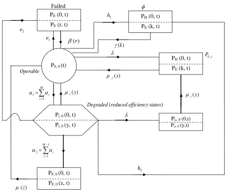
distribution system and it contains N- non-identical units (as shown in fig. 1) connected in series. The subsystem A is of 1-out of N:F nature. The state-transition diagram has shown in fig.2. Some important reliability parameters together with a numerical example and graphical illustrations have appended at the end to show the practical utility of the model.
II. ASSUMPTIONS
The following assumptions are associated with this model:
(1) Initially, all the components are in operable condition of full efficiency.
(2) Failures are statistically independent.
(3) The subsystem B is of nature 1-out-of –M: D.
(4) All the failures follow exponential time distribution where as all the repairs follow general time distribution.
(5) System may be fail due to environmental reasons and human error.
(6) Repair facilities are always available.
(7) After repair system works like a new one and
never damages anything.
(8)
III. NOTATIONS
The following notations have been used throughout this model:
109 Fig.1 (System Configuration)
1
2
3
4
Transmission Substations
Transmission Lines
Power Substations
Transformer Power Poles
110 Fig. 2. State-transition Diagram
P0,j(x,t)∆/Pi,F(y,t)∆ :The probability that at time ‘t’ the system is in failed state due to failure
of (jth-B)/(ith-A and jth-B) component and elapsed repair time lies in the interval (x, x+∆) / (y, y+∆) .
Pi,0(y,t)∆/PF,0(z,t)∆ :The probability that at time ‘t’ , the system is in degraded/failed state due
to failure of ith
–A/2-A components and elapsed repair time lies in the interval (y, y+∆) /(z, z+∆) .
j
P0,
Operable
) (reducedefficiencystates Degraded
∑
−= = 1
1 2
M
i i
α α
∑
= = M
i i
1
1 α
α µi(y)
1 e
2 h
λ
) (y
i
µ λ
) (x
j
µ
) (k
γ
Failed φ
Pi, 0 (0, t)
Pi, 0 (y, t)
P0, 0 (t)
PE (0, t)
PE (r, t)
PH (0, t)
PE (k, t)
1 h
PH (0, t)
PE (k, t)
PF, 0 (0, t)
PF, 0 (z, t)
Pi, F (0,t)
Pi, F (y,t)
) (z
µ 2 e
111 PE(r,t)∆/PH(k,t)∆ :The probability that at time ‘t’, the system is in failed state due to
environmental reasons/human error and elapsed repair time lies in the interval (r, r+∆)/(k, k+∆).
αi/λj : Failure rate of ith-A/jth-B component.
e1/e2
h
: Failure rate due to environmental reasons.
1/h2
β(r)∆/γ(k)∆ : Probability that system will be repaired from environmental failure/human error in time interval (r, r+∆)/(k, k+∆) conditioned that it was not repaired up to time r/k.
: Failure rate due to human error.
µi(y)∆/ µj(x)∆/ µ(z)∆: Probability that ith-A/jth
) (s F
-B/2A components will be repaired in the time interval (y, y+∆)/(x, x+∆)/(z, z+∆) , conditioned that it was not repaired up to the time y/x/z.
: Laplace transform of the function F(t).
Pup(t)/ Pdown(t) : Probability that at time t , the system is in up/down state.
IV. FORMULATION OF MATHEMATICAL MODEL
By the elementary probability consideration and continuity argument, we may obtain the following set of difference-differential equations for the stochastic process, which is continuous in time and discrete in space:
+ +
+ =
+ + + +
∫
∫
∫
∞ ∞∞
dk k t k P dy y t y P dx x t x P t P h e dt
d
H i
i j
j( , ) ( ) ( , ) ( ) ( , ) ( )
) (
0 0
0 , 0
, 0 0
, 0 1 1
1 µ µ γ
α λ
dz z t z P dr r t r
PE( , ) ( ) F ( , ) ( )
0 0 , 0
µ
β
∫
∫
∞∞
+ (1)
0 ) , ( )
( 0, =
+
∂ ∂ + ∂
∂
t x P x t
x µj j (2) 0
) , ( )
( ,0
2 2
2 =
+ + + + + ∂
∂ + ∂
∂
t y P y e
h t
y α λ µi i (3) 0
) , ( )
( ,0 =
+
∂ ∂ + ∂
∂
t z P z t
z µ F (4) )
, ( )
, ( )
(y P, y t P,0 y t t
y µi iF =λ i
+ ∂
∂ + ∂
∂
(5) 0
) , ( )
( =
+
∂ ∂ + ∂
∂
t r P r t
r β E (6) 0
) , ( )
( =
+
∂ ∂ + ∂
∂
t k P k t
112 Boundary Conditions are
dy y t y P t P t
P j(0, ) ( ) iF( , ) i( )
0 , 0 , 0 ,
0 λ
∫
µ∞ +
= (8)
) ( )
, 0
( 1 0,0
0
, t P t
Pi =α (9) )
( )
, 0
( 2 ,0
0
, t P t
PF =α i (10)
0 ) , 0 (
, t =
PiF (11) ) ( ) ( ) , 0
( t e1 P0,0 t e2 P,0 t
PE = + i (12)
) ( ) ( ) , 0
( t h1 P0,0 t h2 P,0 t
PH = + i (13) Initial conditions are
1 ) 0 ( 0 , 0 =
P ; Otherwise all state probabilities are zero. (14) V. SOLUTION OF MATHEMATICAL MODEL
Taking Laplace Transforms of equations (1) through (13), subjected to (14) and then on solving them one by one , we may obtained the following Laplace transforms of different state
probabilities: ) ( 0 , 0 s P = ) ( 1 s
A (15)
) ( )}] ( ) ( { 1 [ ) ( )
( 2 2 2
2 2 2
1 ,
0 S s S s h e Dj s
e h s
A s
P j i − i + + + +
+ + + +
= λ α
α λ α λ (16)
[
( )]
) ( )( 1 2 2 2
0
, D s h e
s A s
Pi = α i +λ+α + + (17)
[
( )]
( )) ( )
( 2 2 2
2 1 0
, D s h e D s
s A s
PF = i +λ+α + +
α α (18)
[
( ) ( )]
) )( ( )( 2 2 2
2 2 2
1
, D s D s h e
e h s
A s
PiF i − i + + + +
+ + +
= λ α
α λ λα (19) ) ( )] ( [ ) ( 1 )
( e1 e2 1D s 2 h2 e2 D s
s A s
PE = + α i +λ+α + + β (20)
) ( )] ( )[ ( )
(s P0,0 s h1 h2 1D s 2 h2 e2 D s
PH = + α i +λ+α + + γ (21)
where, B B S B D A A ) ( 1 )
( = − , for all A and B.
and A(s)= s+λ+α1+h1+e1-α1 Si (s+λ+α2+h2+e2)
) ( )}] ( ) ( { 1
[ 2 2 2
2 2 2
1 S s S s h e S s
e
h + i − i + + + + j
+ + +
− λ α
α λ
α
λ
-α1α2Di(s+λ+α2 +h2+e2)S(s)
- [e1+e2α1Di(s+λ+α2+h2 +e2)]Sβ(s)
113 Also, it is interesting to note that
) ( 0 ,
0 s
P +P0,j(s)+
s s P s P s P s P s
Pi F iF E H
1 ) ( ) ( ) ( ) ( )
( ,0 ,
0
, + + + + = (23)
VI. STEADY-STATE BEHAVIOR OF THE SYSTEM
By using Abel’s lemma, viz; sP s P t P
t
s→ ( )=lim→∞ ( )=
lim
0 (say) ;Provided the limit on R.H.S. exist,
we have the following time independent state probabilities from equations (15) through (21): ) 0 ( 1 0 , 0 A P ′
= (24)
Tj e h S e h A
P j [1 {1 i( )}]
) 0
( 2 2 2 2 2 2
1 ,
0 = ′ +λ+α + + − λ+α + +
α λ (25)
[
( )]
) 0( 2 2 2
1 0
, D h e
A
Pi = ′ i λ+α + +
α
(26)
[
D h e]
TA
PF i( )
) 0
( 2 2 2
2 1 0
, = ′ λ+α + +
α α (27)
[
( )]
) )( 0( 2 2 2 2 2 2
1
, T D h e
e h A
PiF i− i + + +
+ + + ′
= λ α
α λ λα (28) β α λ
α D h e T
e e A
PE [ i( )]
) 0 ( 1 2 2 2 1 2
1+ + + +
′
= (29)
γ α
λ
α D h e T
h h A
PH [ i( )]
) 0 ( 1 2 2 2 1 2
1+ + + +
′
= (30)
where, 0 ) ( ) 0 ( = = ′ s s A ds d
A and Tj =−Si'(0)etc.
VII. PARTICULAR CASE
When all the repairs follow exponential time distribution
Setting Si(s)= i i
s µ µ
+ etc. in equations (15) through (21), we obtain the following Laplace
transforms of various state probabilities:
) ( 0 , 0 s P = ) ( 1 s
B (31)
i i i i i j s e h s s e h s B s P µ µ α λ µ µ µ α λ α λ + + + + + + − + + + + +
= [1 { }] 1
) ( ) ( 2 2 2 2 2 2 1 ,
0 (32)
i i
e
h
s
s
B
s
P
µ
α
λ
α
+
+
+
+
+
=
2 2 2 1 0 ,1
)
(
)
114 ) )( ( 1 ) ( ) ( 2 2 2 2 1 0
, λ α µ µ
α α + + + + + + = s e h s s B s P i
F (34)
+ + + + + − + + + + = i i F i e h s s e h s B s P µ α λ µ α λ λα 2 2 2 2 2 2 1 , 1 1 ) )( ( )
( (35)
1 2 1 [ ) ( 1 )
( e eα
s B s
PE = +
i
e h
s+λ+α2+ 2 + 2+µ 1 ] β + s 1 (36) 1 2 1 [ ) ( 1 )
( h hα
s B s
PH = +
i
e h
s+λ+α2+ 2+ 2+µ 1 ] γ + s 1 (37) where,
B(s)= s+λ+α1+h1+e1
-i i
e h
s λ α µ
µ α + + + +
+ 2 1 2 2 − [1+λ+α2 +1h2+e2 α λ + + + + + −
+i i s ih e i
s λ α µ
µ µ µ 2 2 2 ] j j s µ µ + µ µ µ α λ α α + + + + + + − s e h
s 2 2 2 i
2 1 β β µ α λ α + + + + + + + − s e h s e e i 2 2 2 1 2 1 1 γ γ µ α λ λ + + + + + + + − s e h s h h i 2 2 2 1 2
1 (38)
VIII. UP AND DOWN STATE PROBABILITIES
We have } ) ( exp{ } ) ( exp{ ) 1 ( )
(t c 1 e1 h1 t c 2 h2 e2 t
PUp = + − λ+α + + − − λ+α + + (39) where, C=
1 1 1 2 2 2 1 e h e
h + − − −
+ α
α
α
(40) Also, Pdown(t)=1−PUp(t) (41)
IX. PROFIT FUNCTION
The profit function for the considered system is given by 3
0
2
1 ( )
)
(t C P t dt C t C
G
t
Up − −
=
∫
where, C1 and C2 are revenue and repair costs per unit time and C3
{
}
{
}
2 3) ( 2 2 2 ) ( 1 1 1 1 2 2 2 1 1 1 1 1 1 )
( e Ct C
e h C e h e C C t
G e h t h e t − −
− + + + − − + + + +
= −λ+α + + −λ+α + +
α λ α
λ
is system establishment cost per set up. So, have
115 X. NUMERICAL COMPUTATION
For a numerical comput ation, let us consider the values:
time unit per Rs
C h
h e
e 0.01, 0.02, 0.03, 0.035, .7.00 ,
07 . 0 , 06 . 0 , 001 .
0 1= 2 = 1 = 2 = 1= 2 = 1 =
= α α
λ
C2 = Rs. 2.00 per unit time , C3
By using these values in equations (39),(41) and (42), we may observe the changes in values of corresponding reliability parameters.
= Rs. 10.00 per set up and t = 0,1,2 .. .. .. .. .. ..
where C= 2.4
025 .
06 . 1 . 125 .
06
. = =
−
PUp(t)=3.4 e-0.101t -2.4 e-0.126t
{
}
{
1}
2 10126 .
4 . 2 1
101 .
4 . 3 7 )
(t = −e−.101 − −e−0.126 − t−
G t
and
XI. RESULTS & DISCUSSION
In this model, the authors have evaluated availability and profit function for a power distribution system. Since the system is of non-Markovian nature, the supplementary variables have been introduced to make the system Markovian. These supplementary variables disappear at the solution stage.
We compute the table-1 and 2 for the considered numerical example. The corresponding graphs have shown in the fig-3 and 4. Table-1 shows that how the availability of the power plant decreases as we make increase in the value of time. Availability decreases approximately in a constant manner.
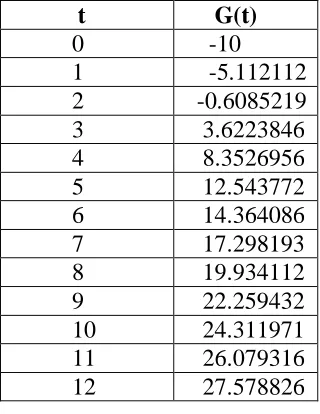
From table-2 we observe that from t= 0 to 2 the profit function is negative. This shows that there is no profit up to t=2 because initially we only have to spend money to establish the system and initial repairs. After t=2 , we recover the system establishment cost and so it becomes positive. Thus after t=2 profit function increases in uniform way.
0 0.2 0.4 0.6 0.8 1 1.2
0 1 2 3 4 5 6 7 8 9 10 11 12
Pup(t)
Table-1
t
Fig 3 t PUp(t)
0 1.0 1 0.9568 2 0.91286 3 0.86644 4 0.80536 5 0.74786 6 0.7279 7 0.68318 8 0.63962 9 0.59778 10 0.5574 11 0.51904 12 0.48264
116
-15 -10 -5 0 5 10 15 20 25 30
0 1 2 3 4 5 6 7 8 9 10 11 12
G(t)
t Fig 4
Table-2
REFERENCES
[1] Cassady, C.R.; Lyoob, I.M.; Schneider, K.; Pohi, E.A. : “A generic model of equipment availability under imperfect maintenance”, IEEE TR. On reliability, vol.54, issue-4, PP. 564-571, 2005.
[2] Fang-Ming, S.; Xuemin, S.; Pin-Han, H.: “Reliability optimization of distributed access networks with constrained total cost’’, IEEE TR. on reliability, vol.54, Issue-3, PP 421-430, 2005.
[3] Sim, S.H.; Endrenyi, J.: “A failure-repair model with minimal and major maintenance”, IEEE TR. on reliability, vol.55, issue-1, P.P. 134-140, 2006.
[4] Wang, F.K.: “Quality evaluation of a manufactured product with multiple characteristics” , Quality and Reliability engineering , vol. 22, issue-2, P.P.225-236,2006.
t G(t) 0 -10 1 -5.112112 2 -0.6085219 3 3.6223846 4 8.3526956 5 12.543772 6 14.364086 7 17.298193 8 19.934112 9 22.259432 10 24.311971 11 26.079316 12 27.578826
G(t)