The Thirty-Third AAAI Conference on Artificial Intelligence (AAAI-19)
Counting and Sampling Markov Equivalent Directed Acyclic Graphs
Topi Talvitie
Department of Computer Science University of Helsinki [email protected]
Mikko Koivisto
Department of Computer ScienceUniversity of Helsinki [email protected]
Abstract
Exploring directed acyclic graphs (DAGs) in a Markov equiv-alence class is pivotal to infer causal effects or to dis-cover the causal DAG via appropriate interventional data. We consider counting and uniform sampling of DAGs that are Markov equivalent to a given DAG. These problems effi-ciently reduce to counting the moral acyclic orientations of a given undirected connected chordal graph onnvertices, for which we give two algorithms. Our first algorithm requires O(2nn4)arithmetic operations, improving a previous super-exponential upper bound. The second requiresO k! 2kk2n
operations, wherek is the size of the largest clique in the graph; for bounded-degree graphs this bound is linear inn. After a single run, both algorithms enable uniform sampling from the equivalence class at a computational cost linear in the graph size. Empirical results indicate that our algorithms are superior to previously presented algorithms over a range of inputs; graphs with hundreds of vertices and thousands of edges are processed in a second on a desktop computer.
1
Introduction
In causal discovery a key task is to learn adirected acyclic graph (DAG)on the variables of interest. What makes learn-ing particularly challenglearn-ing is that different DAGs can repre-sent the same conditional independence relations among the variables; such DAGs areMarkov equivalent. Every Markov equivalence class can be represented uniquely by an essen-tial graph(a.k.a.completed partial DAG), in which an edge is undirected unless the direction is unique in the class (An-dersson, Madigan, and Perlman 1997). Purely observational data are generally sufficient for identifying a unique essen-tial graph, but not singling out a DAG.
That said, the DAGs within a given equivalence class are well worth exploring, for instance, to estimate causal effects between pairs of variables (Maathuis, Kalisch, and B¨uhlmann 2009) or to direct some of the undirected edges in the essential graph based on interventional data (Ghas-sami et al. 2018). Such tasks call for efficient algorithms for generating random DAGs from a given equivalence class, as well as, for studying the related combinatorial problem of computing the size of the equivalence class. It is well known that these problems immediately (and efficiently) reduce to
Copyright c2019, Association for the Advancement of Artificial Intelligence (www.aaai.org). All rights reserved.
their restricted variants where the essential graph is an undi-rected connected chordal graph (UCCG); see Gillispie and Perlman (2002) and Section 2. Then the DAGs in the equiv-alence class correspond to what we, in this paper, callmoral acyclic orientations (MAOs).
Two approaches to count and sample MAOs have been investigated recently. For counting, He, Jia, and Yu (2015) discovered a recurrence: by guessing the unique source ver-tex of a MAO (i.e., branching on the options), the orien-tations of some edges get fixed, leaving some number of smaller disjoint UCCGs; if a so-encountered UCCG is an “almost clique,” then a fast special treatment is given. He and Yu (2016) enhanced the algorithm by extracting at every level of the recurrence a so-called core graph of the UCCG in question. Ghassami, Salehkaleybar, and Kiyavash (2018) observed that the basic recurrence admits a complexity boundn∆+O(1)on graphs of maximum degree∆, and
read-ily allows for uniform sampling.1 While these algorithms can handle sparse graphs with hundreds of vertices, their best known worst-case complexity bound is O(n!). Bern-stein and Tetali (2017) took a different approach and consid-ered sampling MAOs from an almost uniform distribution. They showed that a simple edge-flip Markov chain mixes in time that is exponential in the worst case but polynomial under certain restrictions on the input UCCG.
In this paper we give new exact algorithms. Our algo-rithms (i) yield improved worst-case complexity bounds and (ii) also run faster in practice, by several orders of magnitude in some cases. We begin in Section 2 by introducing more formally the problem and the basic recurrence. Then, in Sec-tion 3, we make a simple observaSec-tion that gives us adynamic programming (DP)variant of the recursive algorithm with a complexity bound ofO 2nn4
. In Section 4 we derive a bet-ter bound for sparse graphs. Specifically, we assume that the largest clique has sizek, potentially much smaller thann, and give another DP algorithm that requires O k! 2kk2n
operations. Using standard routines, both algorithms can be turned into uniform samplers. In Section 5 we report on em-pirical results and draw conclusions as to which algorithm is the fastest for what type of instances. We end in Section 6 by discussing open questions and directions for future research.
1
c b
e
g h
f d
a
(a) DAG
c b
e
g h
f d
a
(b) Essential graph
c b
e
g h
f d
a
(c) UCCGs
c b
e f
d
a
(d)e-orientation
c b
e f
d
a
(e) Subproblem
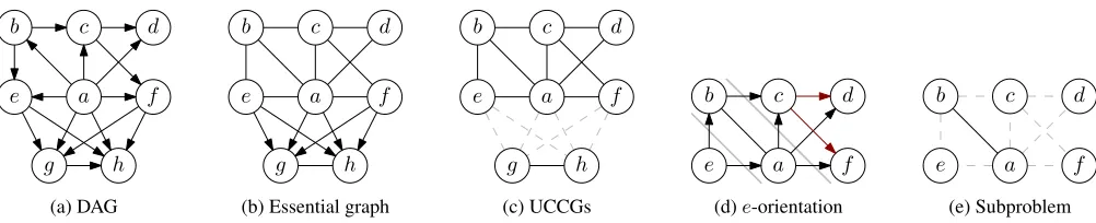
Figure 1: Illustration of some key concepts. (a) A DAG, (b) its essential graph, (c) the UCCG components of the essential graph. (d) Thee-orientation of the larger UCCG. In addition to orienting the edges between vertices at different distances frome, we also orientc→dandc→fbecause otherwise we would get new immoralitiesb→c←dandb→c←f, respectively. (e) The remaining subproblem after removing directed edges.
2
Preliminaries
We will need a number of concepts and terminology, some of which are rather standard in graph theory, and others that are more specific and developed in the literature on Markov equivalence classes (Andersson, Madigan, and Perl-man 1997). This section also reviews the basic recurrence discovered by He, Jia, and Yu (2015).
Basic Graph Terminology
A graph is a pairG = (V, E)with a finitevertex setV and an edge setE ⊆ V ×V \ {vv : v ∈ V}. Between two verticesu, v there is anundirected edge, called lineu−v, ifuv, vu ∈ E, and adirected edge, calledarrowu→v, if
uv ∈ Ebutvu 6∈ E. The graph isundirected(directed) if all its edges are undirected (resp. directed).
A graph(S, F)is asubgraphofGandcontainedinG if
S⊆V andF ⊆E∩(S×S); it isspanning(induced) if the former (resp. latter) inclusion is an equality. We writeG[S]
for the subgraph ofGinduced byS.
A graph is adirected cycle(undirected cycle) oflength`
if its vertices can be ordered asv0, v1, . . . , v`−1such that its
edges arevi−1→vi(resp.vi−1−vi) for1 ≤i≤`, where
v` = v0. A graph is animmorality(a.k.a.v-structure) if its
vertices can be labeled asu, v, w such that the edge set is
{uv, wv}, i.e., the graph isu→v←w(“the parents ofvare unmarried”). A graph is aflagif its vertices can be labeled as
u, v, wsuch that the edge set is{uv, vw, wv}, i.e., the graph isu→v−w.
A graph isacyclicif it contains no directed cycle of length larger than two,moralif no induced subgraph is an immoral-ity, andchordalif it is undirected and no subset of four or more vertices induces an undirected cycle.
A graphGis achain graphif it does not contain a semi-directed cycle, that is, a subgraph that is a semi-directed cycle with at least one arrowu→vsuch thatu−vis a line inG. Achain component (CC) of a chain graph is a connected component of the undirected graph obtained by removing all directed edges.
Markov Equivalence Classes
LetD= (V, A)be a DAG. Theessential graphofDis the graphE = (V, E), whereE is the union of the edge sets of the DAGs that are Markov equivalent toD(Andersson,
Madigan, and Perlman 1997). Thus the essential graph is a unique representation of the Markov equivalence class. The essential graph can be constructed efficiently (Meek 1995).
It is known that an essential graph is a chain graph where each CC is an undirected and connected chordal graph (UCCG)(Andersson, Madigan, and Perlman 1997). The ver-tex sets of the CCs,V1, V2, . . . , Vc, partitionV. Denoting by µ(E)the size of the Markov equivalence class represented byE, we thus have that (Gillispie and Perlman 2002)
µ(E) =
c
Y
i=1
µ(E[Vi]). (1)
In other words, the equivalence class represented byEand a Cartesian product of the equivalence classes represented by each chain component are in one-to-one correspondence.
Figure 1(a–c) shows an example of a DAG, the corre-sponding essential graph, and its UCCG components.
Moral Acyclic Orientations
The above observations motivate focusing on the problems of counting and sampling DAGs that belong to the equiva-lence class represented by a given UCCGC. Each such DAG is anorientationofC, that is, a spanning subgraph that con-tains exactly one of the arrowsu→v andv→ufor every lineu−vinC; furthermore, the orientation must be moral. It is easy to see that themoral acyclic orientations (MAOs)
are exactly the members of the equivalence class (He, Jia, and Yu 2015). Our key problem is thus the following:
#MAO
Input:Ann-vertex UCCGC= (V, E).
Output:The number of MAOs ofC, i.e.,µ(C).
The Sum–Product Recurrence
It is known that every MAO of a UCCG has a unique source vertex. He, Jia, and Yu (2015) observed that the MAOs with a fixed source vertex s agree on the orientation of some edges, while the remaining edges again leave an undirected chordal subgraph. They call the union of the MAOs an s-rooted essential graph; we use the term s-orientation for brevity and because the graph may not be an essential graph. Definition 1. Let C be a UCCG with vertex s. The s-orientation ofC, denoted byCs, is the union of all MAOs
Since ans-orientation is a chain graph whose chain com-ponents are UCCGs (He, Jia, and Yu 2015, Thm. 7),
µ(C) =X
s∈V µ(Cs),
where eachµ(Cs)admits again the product rule (1).
To construct ans-orientation of a UCCGC, He, Jia, and Yu (2015) give the following algorithm (sligthly modified):
AlgorithmOrient: (C, s)7→ Cs
O1 CreateC0by orienting each lineu−vofCasu→vifs is closer touthanvinC(in the shortest-path distance).
O2 As long asC0has a flagu→v−was an induced sub-graph, updateC0by orientingv−wasv→w.
O3 OutputC0.
Figure 1(d–e) shows an example of ans-orientation and the resulting subproblems.
3
Dynamic Programming
We will make a simple but crucial observation, which shows that the number of distinct subproblems encountered by the sum–product recurrence is at most2n, wheren=|V|is the
number of vertices of the input UCCG. We will do this by showing that every subproblem corresponds to aninduced
subgraph of the input UCCG.
Let us first consider a single step in the recurrence.
Lemma 1. LetC be a UCCG with a vertexs. LetI be a chain component ofCs. ThenIis an induced subgraph ofC.
Proof. We have thatI is an induced subgraph ofCsand a
UCCG (He, Jia, and Yu 2015, Thm. 7). SinceCs is a
sub-graph ofC(obtained by removing some edges), it suffices to show that two verticesuandvare non-adjacent inIonly if they are non-adjacent inC. But this is immediate, as inCthe two vertices are either non-adjacent or connected by a line, which is either unchanged or directed inCs.
Encouraged by this observation we letµC(S) :=µ(C[S]) forS⊆V. In particular,µC(V)is the number of MAOs of C. We next show that this function satisfies a sum–product recurrence analogous to the one for UCCGs.
Proposition 2. LetC be a UCCG and S its vertex subset that induces an UCCGC˜:=C[S]. We have that
µC(S) =
X
s∈S
Y
T
µC(T),
whereT runs through the vertex sets of the CCs ofC˜s, the s-orientation ofC[S].
Proof. By the recurrence of He, Jia, and Yu (2015) we have that
µ( ˜C) =X
s∈S
Y
T
µ( ˜Cs[T]),
whereT ranges as in the statement. By Lemma 1, we have thatC˜s[T] = ˜C[T]. It remains to observe thatC[˜T] =C[T],
forT ⊆S(by basic properties of induced subgraphs).
Proposition 2 suggests a dynamic programming algorithm that computes and stores the value µC(S)using the recur-rence at most once for each S. Because potentially only a small fraction of all subsets need be evaluated, we propose a top-down, recursive implementation with memoization: AlgorithmMemoMao: C 7→µ(C)
M1 Leta[·]be a storage indexed byS ⊆V; initiallya[S]
returns1ifSis a singleton, andNULLotherwise. M2 OutputSum-Product(V).
FunctionSum-Product(S)
S1 Ifa[S]6=NULL, returna[S]; else leta[S]←0. S2 For each vertexs∈S:
• RunOrientto getC0, thes-orientation ofC[S]. • Let(Si)ci=1be the vertex sets of the CCs ofC0.
• Leta[S]←a[S] +Qc
i=1Sum-Product(Si).
S3 Returna[S].
The main result of this section now follows. Theorem 3. The complexity of#MAOisO(2nn4).
Proof. Clearly it suffices to estimate the cost of step S2 of FunctionSum-Product. Consider an arbitrary subsetSofV. By step S1 we have that S2 is run at most once for eachS. One S2 needsO(|S|)additions andO(|S|2)multiplications.
To bound the number of other operations, required for constructing eachs-orientation and its component UCCGs, consider a fixed s ∈ S. The lengths of the single-source shortest paths and thus step O1 of Algorithm Orient can be computed withO(n2)operations. Step O2 is seen to re-quireO(n3)operations, by the following argument: for each
linev−woriented asv→w, it suffices to consider once the neighboringO(n)lines of the formw−xand test whether
vandxare adjacent (byv→x).
Thus O(n4) operations suffice for any fixed S, and
O(2nn4)operations in total.
Remark 1 (Bit complexity). The proof shows that other operations than additions and multiplications dominate the complexity bound, implying that the bit complexity of
#MAO is at most2nn4up to a factor logarithmic inn.
Remark 2(Uniform sampling). In order to support efficient uniform sampling of MAOs, for each encountered set S, we store the constructed s-orientations and associate each with the respective weight (i.e., the product) in the sum– product formula. To enable constant-time sampling of an
s-orientation with a probability proportional to its weight, we use the alias method (Walker 1977; Vose 1991). Starting fromS=V and proceeding recursively into the component UCCGs, we can draw a random DAG inO(|V|+|E|)time.
4
Using Tree Decomposition
Cliques and Tree Decomposition
A tree decomposition (TD)of a graph (V, E)is a tree T
where eachnodexis labelled by abagBx⊆V such that (i)
the endpoints of each edgeuv∈Eoccur in one of the bags, and (ii) for each vertexv∈V the nodes whose bag contains
vinduce a non-empty connected subtree ofT. Thewidthof the tree decomposition is size of the largest bag minus one.
Chordal graphs are special in that they admit a TD, called
clique tree, whose bags are exactly the maximal cliques of the graph (Blair and Peyton 1993). Such a decomposition is optimal in the sense that no TD can have a smaller width. Furthermore, one can construct a clique tree in time linear in the graph size (Blair and Peyton 1993). Another useful prop-erty of a clique tree is that the underlying graph is obtained as itsintersection graph, that is, by connecting two vertices by an edge if and only if they both appear in same bag. We will use this property to relate a MAO ofCto a collection of linear orders on the bags of a TD ofC.
Definition 2. LetCbe a UCCG andT its TD where the bag
Bxof each nodexis a clique ofC. Assign each nodexofT
a linear order≺xonBx. The assignment isfriendlytoT if
the following holds for all adjacent nodesx, y:
(f1) The orders≺x and ≺y are compatible, i.e., they are
equal when restricted toBx∩By.
(f2) LetX 3 xandY 3 y be the components ofT that remain after disconnectingxandy. For any vertexv ∈
Bx∩By, at most one of the following cases holds:
• For some nodez ∈ X the bagBzcontainsvand
an-other vertexusuch thatu≺zvandu6∈By.
• For some nodez ∈ Y the bagBz containsvand an-other vertexusuch thatu≺zvandu6∈Bx.
Lemma 4. The MAOs of C are in one-to-one correspon-dence with the linear order assignments friendly toT.
Proof. Consider first a MAOA of C. For each nodexof
T, let≺x be the edge set of the induced subgraphA[Bx].
Clearly, the assignment(≺x)xis unique. We need to show
that conditions (f1) and (f2) are satisfied. The former is ob-vious. To check the latter condition, let x, y be adjacent nodes and X, Y as in the statement of the condition. Let
v∈Bx∩By. Now, if both cases of (f2) hold, then there
ex-ist verticesuandu0suchAhas the arrowsu→vandv←u0
even ifuareu0are not adjacent inC. ThusAcontains an im-morality, which is a contradiction, as desired.
For the other direction, let(≺x)xbe a linear order
assign-ment that is friendly toT. Because of the property (ii) of the definition of TD, friendliness condition (f1) also holds for non-adjacent nodesx, y. Thus the linear orders determine a unique orientationDofC: orient an edgeuvas u→v if
u, v ∈ Bxandu≺x vfor somex. It remains to show that
Dis moral and acyclic. For the former, assume the contrary, i.e., there is an immoralityu→v←u0. Then there must be adjacent nodesx, ysuch thatv ∈ Bx∩By,u∈Bx\By, u0 ∈ By\Bx. This violates (f2), implyingDis moral. To show acyclicity, assume the contrary:Dcontains a cycle. We can assume thatu→v→w→uis the cycle, because if it is longer, by the chordality ofCwe know that there is a short-cut edge, and we can shorten the cycle. Letx, y, zbe nodes
ofT such that{v, w} ⊂ Bx,{w, u} ⊂ By,{u, v} ⊂ Bz. BecauseT is a tree, the three unique simple paths fromx
toy,ytoz, andz toxall pass through a common nodec. By the definition of TD, we have that{u, v, w} ⊂Bc. Thus it holds thatu≺c v ≺c w ≺c u, which is a contradiction
because≺cis a linear order. ThusDis acyclic.
The Algorithm
Lemma 4 allows us to formulate the DP algorithm in the space of (friendly) assignments of linear orders on the bags of a TD. For writing the DP steps, it will be convenient to assume that T is a nice TD, that is, when rooted at some noder, each nodexis of one of the following types:
Leaf: no children.
Introduce: one child y, introduces a v ∈ V \ Bx, i.e.,
By=Bx∪ {v}.
Forget: one childy, forgets av∈Bx, i.e.,By=Bx\{v}.
Join: two childreny, z, withBx=By=Bz.
On a high level, the algorithm employs DP over the sub-trees of a nice TD. For each subtree rooted at nodex, it com-putes a tableFxbased on the tablesFyof the childreny of x. Finally,µ(C)is extracted from the tableFrat the root.
Define the tableFxfor each nodexas follows. LetX be
the set of nodes in the subtree rooted atx. For every linear order ≺on Bx and subset P ⊆ Bx, define Fx(≺, P) as
the number of assignments of linear orders≺y onBy, for y∈X, such that the following conditions hold:
• The assignment(≺y)y∈Xis friendly toT[X].
• The linear order≺xis equal to≺.
• The set P consists of exactly those vertices in Bx that have a predecessor in some node of the subtree that is not present inBx(alost predecessor), i.e.,
P=[
y∈X
v∈By∩Bx:u≺yvfor someu∈By\Bx .
We will needP to satisfy the friendliness condition (f2).
By Lemma 4, µ(C)is the sum of the values in the table
Fr. It remains to show how each tableFxis computed from the tables of the child nodes. In the description, we include derivations that prove the correctness of the algorithm, i.e., that the computed values, we denote byFx[≺, P], equal the
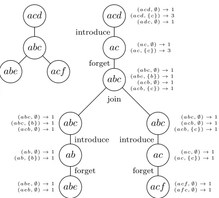
corresponding values,Fx(≺, P). See Figure 2 for an illus-tration of the algorithm.
AlgorithmTreeMao: C 7→µ(C)
T1 LetT be a nice TD ofC, rooted atr.
T2 For each nodexofT, from the leaves towards the root, initialize the tableFx[·,·]to zero, and then populate it:
• Ifxis a leaf node: Since the subtree has only one clique,
Bx, all linear orders are possible and there are no lost predecessors. Thus we letFx[≺,∅] ← 1for all linear
• Ifxintroduces vertexv: Lety be the child of x, and consider all the elementsFy(≺, P). The only way to extend the assignment of linear orders fromX\ {x}to
X, satisfying condition (f1), is by the linear order ≺0 obtained from≺by removing vertexv. Condition (f2) cannot be violated by this extension. After the removal ofv, we need to add all of its successors in≺to the set of vertices with lost predecessors, and thus we increase
Fx[≺0, P ∪ {u∈Bx:v≺u} \ {v})]byFy[≺, P].
• Ifxforgets vertexv: Lety be the child ofx, and con-sider all the elementsFy(≺, P). To extend the assign-ment of linear orders fromX \ {x} toX, by condi-tion (f1), we only need to consider the|Bx| possible linear orders≺0 obtained from≺by adding vertexv. To satisfy condition (f2), it must hold that there is no predecessoru∈Bysuch thatu≺0vthat is also inP. Thus we increaseFx[≺0, P]byFy[≺, P].
• Ifxjoins nodesy andz: LetY andZ the nodes sets of the subtrees rooted atyandz, respectively. Because
Bx = By = Bz, every assignment of linear orders
toXis obtained by combining assignments(≺w)w∈Y
and(≺w)w∈Z where≺y=≺z, and letting≺x← ≺y.
To satisfy condition (f2), we only need to ensure that the sets of vertices with lost predecessors fromY andZ
are disjoint, and in the combined assignment, the set of lost predecessors is obtained as the disjoint union. Thus we letFx[≺, P]←PS⊆PFy[≺, S]·Fz[≺, P \S].
T3 OutputP
≺,PFr[≺, P].
We are ready to prove the main result of this section: a parameterized complexity bound for#MAO:
Theorem 5. TreeMao requires O(k! 2kk2n) operations,
wherekis the size of the largest clique in the input graph.
Proof. Constructing a clique tree requires O(nk2)
opera-tions, linear in the size of the input. The clique tree hasO(n)
nodes and widthk−1. It is transformed inO(nk2)
opera-tions into a nice TD withO(n)nodes and widthk−1 (Bod-laender, Bonsma, and Lokshtanov 2013). Thus the complex-ity of step T1 is dominated by the bound being proven.
Each table Fx containsO(k! 2k) elements. It is easy to
see that for leaf, introduce and forget nodes, the computa-tions takeO(k2)operations per element. For a join nodex, we get the subtable Fx[≺,·] from the subtables Fy[≺,·]
andFz[≺,·]as the so-calledsubset convolution. Using fast subset convolution it also costs k2 operations per element
(Bj¨orklund et al. 2007, Thm. 1). Now, because there are
O(n)nodes, we get the claimed complexity bound.
Practical Tricks
The DP algorithm described above was designed to optimize the upper bound for the worst-case asymptotic complexity. In applications, however, we care more about the actual run-ning time. We next describe some optimizations in our im-plementation that improve the running time in practice.
While a nice TD simplifies the description of the algo-rithm, for practical performance it is better to implement in-troducing, forgetting and joining in a single operation one
ab abc
acf ac abc abc
ac acd
abe forget
introduce introduce
forget join forget introduce acd
abc
abe acf
(ac,∅)→1 (ac,{c})→1
(acf,∅)→1 (af c,∅)→1 (abe,∅)→1
(aeb,∅)→1 (ab,∅)→1 (ab,{b})→1 (abc,∅)→1 (abc,{b})→1 (acb,∅)→1
(abc,∅)→1 (acb,∅)→1 (acb,{c})→1 (abc,∅)→1
(abc,{b})→1 (acb,∅)→1 (acb,{c})→1 (ac,∅)→1 (ac,{c})→3 (acd,∅)→1 (acd,{c})→3 (adc,∅)→1
Figure 2: A tree decomposition and a nice tree decomposi-tion for the larger UCCG in Figure 1(c). For each node, the portion of the dynamic programming table where ais the first vertex of the linear order is shown.
a clique tree. This way the TD has the minimum number of nodes and the tables can be kept as small as possible by forgetting vertices that do not appear outside the subtree.
To obtain the complexity bound in Theorem 5, fast subset convolution was crucial in join operations. Our preliminary experiments showed that, in practice, the subtablesFx[≺,·]
are often so sparse that a simple enumeration of all pairs of nonzero elements in the child subtablesFy[≺,·]andFz[≺,·]
and filtering out the cases where the arguments (i.e., vertex subsets) intersect is faster than fast subset convolution. For this to work, we store the tables in a way that allows for sparsity, e.g., with balanced binary trees or hash tables.
In dense graphs some vertices tend to be symmetric: they appear in the bags of exactly the same nodes, at least in sub-trees. Symmetric vertices are interchangeable in the DP ta-bles, and we save space and computation time by storing the symmetric elements in the table only once.
Remark 3 (Sampling). The computed tables enable effi-cient sampling of MAOs (cf. Remark 2). The only difficulty is that for join nodes, the counting algorithm uses fast subset convolution, which we cannot directly use for sampling the partition of the setP of lost predecessors for the two chil-dren. However, by enumerating all partitions, we obtain a sample inO(2kn)time. We can also sample inO(|V|+|E|)
time by a variant of the counting algorithm without fast sub-set convolution, yielding a complexity ofO(k!3kk2n).
5
Experiments
We have evaluated four exact algorithms for#MAO:
• MemoMao: The DP algorithm based on the sum–product recurrence (Section 3).
16 32 64 128 256 512 1024
n
0.0001 s 0.001 s 0.01 s 0.1 s 1 s 10 s 100 s 600 s
Running
time
r=4
2 3 4 5 6 8 10 12
r n=32
MemoMao TreeMao He et al. 2015 He & Yu 2016
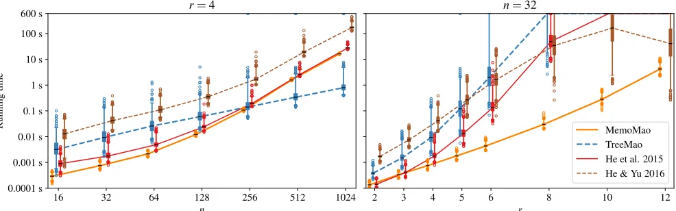
Figure 3: Running times of the four algorithms as functions ofnandron random UCCGs withnvertices andrnedges. The box is between percetiles 25% and 75%; the whiskers are at 1% and 99%.
• He et al. 2015: The algorithm based on the sum–product-recurrence without DP due to He, Jia and Yu (2015).
• He & Yu 2016: Improved version of the previous method based on core graphs (He and Yu 2016).
We implemented all four algorithms in C++2, using only a single thread of execution and exact integer computations.
Extending on the experimental setup from He, Jia and Yu (2015), we run all the algorithms on randomly generated UCCGs withnvertices andrnedges, where16≤n≤1024
and 2 ≤ r ≤ 12. The random generation works in two phases: First we generate a tree by starting from a single vertex and repeatedly adding a vertex as a neighbor of a ran-domly chosen vertex in the current tree until the tree hasn
vertices. After this, we add edges between pairs of vertices chosen uniformly at random, while on each step maintaining the chordality of the graph, until the graph hasrnedges.
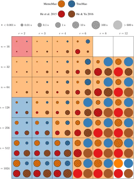
For eachrandn, we generated1000UCCGs and ran each algorithm for every UCCG with time limit of 10 minutes and memory limit of 4 GB. Figure 4 shows the median running times of the algorithm, and Figure 3 shows the ranges of the running times for slicesr= 4andn= 32.
From the results we see thatMemoMaois the fastest al-gorithm in most cases, butTreeMao is faster in sparse in-stances. In the median running times in Figure 4,MemoMao
is faster thanTreeMaowhenn ≤2r+4. The growth of the
running time ofMemoMaoas a function ofris remarkably slow, and the improvement overHe et al. 2015 on which it is based is multiple orders of magnitude for larger. The random fluctuations in the running times ofMemoMaoare also very small.He & Yu 2016does not do particularly well except for very dense instances such asn= 32, r= 12.
6
Concluding Remarks
We have presented two new exact algorithms to count and uniformly sample DAGs that are Markov equivalent to a given DAG. We focused on the core case where the equiv-alence class is represented by an undirected, connected,
2
github.com/ttalvitie/count-mao
and chordal essential graph. Common to both algorithms,
MemoMaoandTreeMao, is a systematic exploitation of the overlapping subproblems structure using dynamic program-ming. The experiments confirmed that the algorithms not only lower the known asymptotic worst-case complexity up-per bounds, but also are faster than previously presented al-gorithms over a range of inputs.
To enhance the DP algorithms, one could seek more effi-cient ways to exploit symmetries, similar to those by He, Jia, and Yu (2015) and He and Yu (2016). Another direction is to implement hybrid methods, for instance, by lettingTreeMao
solve sparse subproblems encountered byMemoMao. Some fundamental theoretical questions remain open. Can one solve#MAO in polynomial time; is it#P-hard? Does the problem admit a fully polynomial randomized ap-proximation scheme (FPRAS)? We find these questions in-triguing, since the related problem of counting acyclic ori-entations is polynomial time for chordal graphs, but hard in general (Vertigan and Welsh 1992), and an FPRAS is only known for some special cases (Bordewich 2004).
n= 16
n= 32
n= 64
n= 128
n= 256
n= 512
n= 1024
r= 2 r= 3 r= 4 r= 6 r= 8 r= 12
MemoMao TreeMao
He et al. 2015 He & Yu 2016
<0.001s 0.01s 0.1s 1s 10s 100s >600s
Acknowledgments
This work was supported in part by the Academy of Finland, under Grant 276864.
References
Andersson, S. A.; Madigan, D.; and Perlman, M. D. 1997. A characterization of Markov equivalence classes for acyclic digraphs. The Annals of Statistics25(2):505–541.
Bernstein, M., and Tetali, P. 2017. On sampling graphical Markov models.ArXiv e-prints 1705.09717.
Bj¨orklund, A.; Husfeldt, T.; Kaski, P.; and Koivisto, M. 2007. Fourier meets M¨obius: Fast subset convolution. In
Proceedings of the 39th ACM Symposium on Theory of Com-puting, 67–74. New York, NY, USA: ACM.
Blair, J. R. S., and Peyton, B. 1993. An introduction to chordal graphs and clique trees. In George, A.; Gilbert, J. R.; and Liu, J. W. H., eds., Graph Theory and Sparse Matrix Computation, 1–29. New York, NY: Springer.
Bodlaender, H. L.; Bonsma, P. S.; and Lokshtanov, D. 2013. The fine details of fast dynamic programming over tree de-compositions. InParameterized and Exact Computation – 8th International Symposium, IPEC 2013, volume 8246 of
Lecture Notes in Computer Science, 41–53. Springer.
Bordewich, M. 2004. Approximating the number of acyclic orientations for a class of sparse graphs. Combinatorics, Probability and Computing13(1):1–16.
Ghassami, A.; Salehkaleybar, S.; Kiyavash, N.; and Barein-boim, E. 2018. Budgeted experiment design for causal struc-ture learning. InProceedings of the 35th International Con-ference on Machine Learning, volume 80 ofProceedings of Machine Learning Research, 1724–1733. PMLR.
Ghassami, A.; Salehkaleybar, S.; and Kiyavash, N. 2018. Counting and uniform sampling from Markov equivalent DAGs.ArXiv e-prints 1802.01239.
Gillispie, S. B., and Perlman, M. D. 2002. The size dis-tribution for Markov equivalence classes of acyclic digraph models.Artificial Intelligence141(1/2):137–155.
He, Y., and Yu, B. 2016. Formulas for counting the sizes of Markov equivalence classes of directed acyclic graphs.
ArXiv e-prints 1610.07921.
He, Y.; Jia, J.; and Yu, B. 2015. Counting and exploring sizes of Markov equivalence classes of directed acyclic graphs.
Journal of Machine Learning Research16:2589–2609. Maathuis, M. H.; Kalisch, M.; and B¨uhlmann, P. 2009. Esti-mating high-dimensional intervention effects from observa-tional data. The Annals of Statistics37(6A):3133–3164.
Meek, C. 1995. Causal inference and causal explanation with background knowledge. InProceedings of the Eleventh Annual Conference on Uncertainty in Artificial Intelligence, 403–410. Morgan Kaufmann.
Radhakrishnan, A.; Solus, L.; and Uhler, C. 2017. Counting Markov equivalence classes by number of immoralities. In
Proceedings of the Thirty-Third Conference on Uncertainty in Artificial Intelligence. AUAI Press.
Steinsky, B. 2003. Enumeration of labelled chain graphs and labelled essential directed acyclic graphs. Discrete Mathe-matics270(1):267–278.
Steinsky, B. 2004. Asymptotic behaviour of the number of labelled essential acyclic digraphs and labelled chain graphs.
Graphs and Combinatorics20(3):399–411.
Steinsky, B. 2013. Enumeration of labelled essential graphs.
Ars Combinatoria111:485–494.
Vertigan, D. L., and Welsh, D. J. A. 1992. The computa-tional complexity of the Tutte plane: the bipartite case. Com-binatorics, Probability and Computing1(2):181–187. Vose, M. 1991. A linear algorithm for generating random numbers with a given distribution. IEEE Transactions on Software Engineering17:972–975.