The Thirty-Third AAAI Conference on Artificial Intelligence (AAAI-19)
Deep Metric Learning by Online Soft Mining and Class-Aware Attention
Xinshao Wang,
1,2Yang Hua,
1Elyor Kodirov,
2Guosheng Hu,
1,2Neil M. Robertson
1,2 1School of Electronics, Electrical Engineering and Computer Science, Queen’s University Belfast, UK2Anyvision Research Team, UK
{xwang39, y.hua, n.robertson}@qub.ac.uk,{elyor, guosheng.hu}@anyvision.co
Abstract
Deep metric learning aims to learn a deep embedding that can capture the semantic similarity of data points. Given the availability of massive training samples, deep metric learn-ing is known to suffer from slow convergence due to a large fraction of trivial samples. Therefore, most existing methods generally resort to sample mining strategies for selecting non-trivial samples to accelerate convergence and improve per-formance. In this work, we identify two critical limitations of the sample mining methods, and provide solutions for both of them. First, previous mining methods assign one binary score to each sample, i.e., dropping or keeping it, so they only se-lects a subset of relevant samples in a mini-batch. Therefore, we propose a novel sample mining method, called Online Soft Mining (OSM), which assigns one continuous score to each sample to make use of all samples in the mini-batch. OSM learns extended manifolds that preserve useful intraclass vari-ances by focusing on more similar positives. Second, the ex-isting methods are easily influenced by outliers as they are generally included in the mined subset. To address this, we introduce Class-Aware Attention (CAA) that assigns little at-tention to abnormal data samples. Furthermore, by combining OSM and CAA, we propose a novel weighted contrastive loss to learn discriminative embeddings. Extensive experiments on two fine-grained visual categorisation datasets and two video-based person re-identification benchmarks show that our method significantly outperforms the state-of-the-art.
Introduction
With success of deep learning, deep metric learning has attracted a great deal of attention and been applied to a wide range of visual tasks such as image retrieval (Wang et al. 2014; Huang, Change Loy, and Tang 2016; Oh Song et al. 2016), face recognition and verification (Schroff, Kalenichenko, and Philbin 2015; Sun et al. 2014; Taig-man et al. 2014), and person re-identification (McLaugh-lin, del Rincon, and Miller 2017; Song et al. 2018). The goal of deep metric learning is to learn a feature embed-ding/representation that captures the semantic similarity of data points in the embedding space such that samples be-longing to the same classes are located closer, while sam-ples belonging to different classes are far away. Various
Copyright c2019, Association for the Advancement of Artificial Intelligence (www.aaai.org). All rights reserved.
deep metric learning methods have been proposed: doublet-based methods with contrastive loss (Oh Song et al. 2016; Hadsell, Chopra, and LeCun 2006; Shi et al. 2016; Yuan, Yang, and Zhang 2017), triplet-based methods with triple loss (Schroff, Kalenichenko, and Philbin 2015; Wang et al. 2014; Chechik et al. 2010; Hoffer and Ailon 2015; Cui et al. 2016), and quadruplet-based methods with double-header hinge loss (Huang, Loy, and Tang 2016). All of them construct pairs (samples) by using several images and intro-duce relative constraints among these pairs.
Compared with classification task, deep metric learning methods deal with much more training samples since all possible combinations of images need to be considered, e.g., quadratically larger samples for contrastive loss and cubically larger samples for triplet loss. Consequently, this yields too slow convergence and poor local optima due to a large fraction of trivial samples, e.g., non-informative samples that can be easily verified and contribute zero to the loss function. To alleviate this, sample mining meth-ods are commonly used to select nontrivial images to ac-celerate convergence and improve performance. Therefore, a variety of sample mining strategies have been studied re-cently (Schroff, Kalenichenko, and Philbin 2015; Oh Song et al. 2016; Wang and Gupta 2015; Simo-Serra et al. 2015; Huang, Loy, and Tang 2016; Yuan, Yang, and Zhang 2017; Shi et al. 2016; Cui et al. 2016).
Despite the popularity of exploiting sample mining in deep metric learning, there are two problems in the existing methods:
(1)Not making full use of all samples in the mini-batch– the first problem concerns with the use of samples in the mini-batch. When most methods perform sample mining, they select samples out of mini-batch, e.g.,hard1 difficult negatives mining (Oh Song et al. 2016). Specifically, they assign one binary score (0 or 1) to each sample in order to ‘drop it’ or ‘keep it’. In this way, some samples which may be useful to some extent are removed and thus only a subset of samples are mined. Therefore they cannot make full use of information in each mini-batch.
(2) Outliers– the second problem arises from outliers.
1
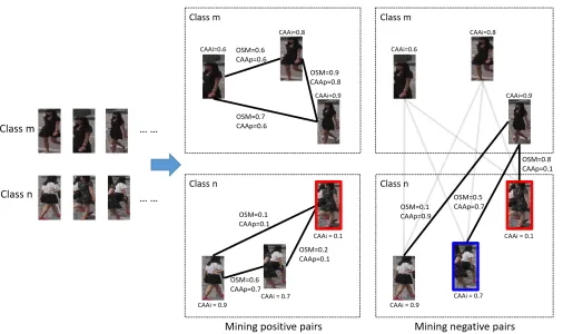
Figure 1: The illustration of Online Soft Mining (OSM) and Class-Aware Attention (CAA) for pair mining. For simplicity, we only consider the scenario with classmand classn. For mining positive pairs, OSM focuses on local positives, i.e., assigning higher scores to the pairs with smaller distance. Meanwhile, CAA helps identify outlier (with red boundary) by CAA score of images (CAAi) and pairs (CAAp). For mining negative pairs (only highlighting pairs of one image from classm), OSM generates higher mining scores for more difficult negatives, e.g., outlier (with red boundary) and true difficult negative (with blue boundary), then CAA helps ignore outliers in the difficult negatives mined by OSM.Best viewed in colour.
The existing mining methods do not consider outliers. How-ever, the presence of noise in the training set hurts the model’s performance significantly as shown in (Zhang et al. 2017). In addition, difficult negatives mining prioritizes samples with larger training loss. As a result, outliers are generally mined in the subset for training as their training losses are more likely to be large.
In this work, we aim to address both problems. Specifi-cally, for the first problem, we propose a novel sample min-ing method, called Online Soft Minmin-ing (OSM), which as-signsone continuous scoreto each sample to make use of all samples in the mini-batch. OSM is based on Euclidean distance in the embedding space. OSM incorporates online soft positives mining and online soft negatives mining. For the positives mining, inspired by (Cui et al. 2016), we as-sign higher mining scores to more similar pairs in terms of distance. This mining has a strong connection to man-ifold learning (Cui et al. 2016), since it preserves helpful intraclass variances like pose and colour in the deep em-bedding space. For the negatives mining,more difficult neg-atives get higher mining scores by soft negatives mining, which can be considered asa generalisation of hard diffi-cult negatives mining(Oh Song et al. 2016; Wang and Gupta
2015; Simo-Serra et al. 2015; Huang, Loy, and Tang 2016; Yuan, Yang, and Zhang 2017; Cui et al. 2016). For the sec-ond problem, we propose Class-Aware Attention (CAA) that
pays less attention to outlying data samples. CAA is sim-ply based on class compatibility score. The illustration of OSM and CAA is given in Figure 1. One attractive prop-erty of OSM and CAA is that they are generic, by which we mean they can be integrated to most existing deep met-ric learning methods (Hadsell, Chopra, and LeCun 2006; Chechik et al. 2010) for mining samples and addressing outliers simultaneously. To demonstrate the effectiveness of OSM and CAA, we propose a novel loss, Weighted Con-trastive Loss (WCL), by integrating them into traditional contrastive loss (Hadsell, Chopra, and LeCun 2006). The weight is assigned to each pair of images defined by OSM and CAA.
pro-posed method’s performance by comparing with other met-ric learning methods on CUB-200-2011 (Wah et al. 2011) and CARS196 (Krause et al. 2013) datasets. For the second one, we use MARS (Zheng et al. 2016) and LPW (Song et al. 2018) datasets, and show that our method surpasses state-of-the-art methods by a large margin.
Related Work
Sample mining in deep metric learning. With the pop-ularity of deep learning (Krizhevsky, Sutskever, and Hinton 2012; Szegedy et al. 2015; Girshick et al. 2016), deep met-ric learning has been widely studied in many visual tasks and achieved promising results (Schroff, Kalenichenko, and Philbin 2015; Oh Song et al. 2016). Compared with tra-ditional metric learning in which hard-crafted features are widely used (Chechik et al. 2010; Weinberger and Saul 2009), deep metric learning learns feature embeddings di-rectly from data points using deep convolutional neural net-works (CNN). Although we can construct a large number of image pairs for deep metric learning, a large fraction of trivial pairs will contribute zero to the loss and gra-dient once the model reaches a reasonable performance. Thus it is intuitive to mine nontrivial pairs during train-ing to achieve faster convergence and better performance. As a result, sample mining has been widely explored and a range of mining methods have been proposed (Schroff, Kalenichenko, and Philbin 2015; Wang and Gupta 2015; Simo-Serra et al. 2015; Huang, Loy, and Tang 2016; Yuan, Yang, and Zhang 2017; Shi et al. 2016; Cui et al. 2016; Oh Song et al. 2016). For mining negatives, mining diffi-cult negatives is applied in (Wang and Gupta 2015; Simo-Serra et al. 2015; Huang, Loy, and Tang 2016; Oh Song et al. 2016). Mining semi-difficult negatives is studied in (Schroff, Kalenichenko, and Philbin 2015; Cui et al. 2016). For mining positives, mining difficult positives is explored in (Simo-Serra et al. 2015; Huang, Loy, and Tang 2016; Yuan, Yang, and Zhang 2017). Mining semi-difficult posi-tives is explored in (Shi et al. 2016). Local posiposi-tives mining (i.e., closer positives) is proposed for learning an extended manifold rather than a contracted hypersphere in (Cui et al. 2016). All of them mine a subset of pairs hardly by us-ing binary score for each pair, i.e., droppus-ing it or keepus-ing it. Instead, our proposed OSM conductssoft mining using continuous score, i.e., assigning different weights for differ-ent pairs. In addition, samples with larger training loss are prioritized when difficult pair mining is applied. Therefore,
outliers are generally mined and perturb the model train-ingdue to their large losses. To address this, semi-difficult negatives mining (Schroff, Kalenichenko, and Philbin 2015; Cui et al. 2016) and multilevel mining (Yuan, Yang, and Zhang 2017) are applied to remove outliers. Instead, we pro-pose CAA for assigning smaller weights to outliers in the mini-batch.
In this paper, following (Sohn 2016; Oh Song et al. 2016; Tadmor et al. 2016), we construct one image pair between every two images in the mini-batch.N-pair-mc loss (Sohn 2016) and Multibatch (Tadmor et al. 2016) treat all the con-structed pairs equally, i.e., without any pair mining. Lifted-Struct (Oh Song et al. 2016) mines most difficult negatives
and treat all positives equally. In contrast, we propose online soft mining for both positives and negatives.
Intraclass variance. In fine-grained recognition (Oh Song et al. 2016; Wah et al. 2011; Krause et al. 2013; Cui et al. 2016) and person re-identification (Zheng et al. 2016; Zhong et al. 2017; McLaughlin, del Rincon, and Miller 2017; Song et al. 2018), intraclass distance could be larger than interclass distance, e.g., images from different cate-gories could have similar colour and shape while the images in the same category can have large variances such as colour, pose and lighting. Several approaches benefit from utilising the inherent structure of data. In particular, local similarity-aware embedding was proposed in (Huang, Loy, and Tang 2016) to preserve local feature structures. (Cui et al. 2016) proposed to learn an extended manifold by using only lo-cal positives rather than treating all positives equally. In a similar spirit with (Cui et al. 2016), our OSM assigns larger weights for more similar positives, intending to learn contin-uous manifolds. The key difference, however, is that a subset composed of local positives are mined in (Cui et al. 2016), whereas our OSM makes use of all positives and gives local positives more attention.
Methodology
Given an image dataset X = {(xi, yi)}, wherexi andyi arei-th image and the corresponding label respectively, our aim is to learn an embedding function (metric)f that takes
xias input and outputs its embeddingfi ∈RD. Ideally, the
learned features of similar pairs are pulled together and fea-tures of dissimilar pairs are pushed away.
Our proposed weighted contrastive loss for learning the embedding functionf is illustrated in Figure 2b. Following the common practice, each mini-batch containsm =c×k
images, wherecis the number of classes andkis the number of images per class. CNN is used for extracting the feature of each image in the mini-batch. In online pair construction, we use all images from the same class to construct posi-tive pairs (i.e., similar pairs) and all images from different classes to construct negative pairs (i.e., dissimilar pairs). As a result, we get m(m−1)/2 image pairs in total. There areck(k−1)/2positive pairs included in the positive set, i.e., P = {(xi,xj)|yi = yj}. Similarly, the negative set,
N ={(xi,xj)|yi6=yj}, consists ofck(ck−k)/2negative pairs. Then, the weight of each pair is generated by OSM and CAA jointly. Our proposed weighted contrastive loss is based on these pairs and their corresponding weights. For reference, the traditional contrastive loss (Hadsell, Chopra, and LeCun 2006) is:
Lαcont(x i
,xj;f) =yijd2ij+(1−yij)max(0, α−dij)2, (1)
where yij = 1 if yi = yj,yij = 0 if yi 6= yj, dij =
kfi−fjk2is the euclidean distance between the pair. It pulls positive pairs as close as possible and pushes negative pairs farther than a pre-defined marginα.
Online Soft Mining
(a) Traditional contrastive loss (b) Weighted contrastive loss with OSM and CAA
Figure 2: The comparison of our proposed weighted contrastive loss with traditional contrastive loss. m is the number of images in a mini-batch. Traditional contrastive loss (a) takes as inputm/2image pairs andm/2binary labels which indicate the corresponding image pair is from the same class or not. Our proposed weighted contrastive loss (b) applies online pair construction. The weighted contrastive loss takes as inputm images and m multi-class labels. We construct non-repeated
m(m−1)/2image pairs online rather than m2pairs in (Oh Song et al. 2016) orm(m−1) pairs in (Tadmor et al. 2016).
Weighted contrastive loss combines Online Soft Mining (OSM) and Class-Aware Attention (CAA) to assign a proper weight for each image pair.
Mining (OSNM) for the negative set.
Online Soft Positives Mining. The goal of OSPM is to generate OSM scores for pairs in the positive set. In many visual tasks, e.g., fine-grained visual categorisation, the interclass distance could be small compared to large in-traclass distance. Motivated by manifold learning in (Cui et al. 2016) wherelocal positives are selected out for learning extended manifolds, OSPM assigns higher OSM scores to local positives. This is because contracted hyperspheres are learned and large intraclass distance cannot be captured if positives with large distance are treated equally.
Specifically, for each similar pair in the positive set, i.e.,
(xi,xj)∈ P, we compute Euclidean distancedij between their features afterL2normalisation. As we want to assign
higher mining scores to more similar pairs, we simply trans-fer the distancedijto OSM score using a Gaussian function with mean=0. In summary, the OSM scores+ij for each pos-itive pair(xi,xj)is obtained as follows:
s+ij = exp(−d2
ij
.
σOSM2) (2)
where dij = kfi − fjk2, σOSM is a hyperparameter for controlling the distribution of OSM scores.
Online Soft Negatives Mining. For dissimilar pairs in the negative set N, we wish to push each pair away by a margin α inspired by the traditional contrastive loss. Similar to previous hard difficult negatives mining meth-ods using binary mining score (Oh Song et al. 2016; Yuan, Yang, and Zhang 2017; Cui et al. 2016; Huang, Loy, and Tang 2016; Ustinova and Lempitsky 2016; Tadmor et al. 2016), to ignore a large fraction of trivial pairs which do not contribute to learning, we assign higher OSM scores to negative pairs whose distance is within this margin. The OSM scores of negative pairs whose distances are larger than the pre-defined margin are set as 0 becausethey do not contribute to the loss and gradient. For simplicity, the OSM scores−ij of each negative pair(xi,xj) is computed directly by the margin distance:
s−ij = max(0, α−dij) (3)
Class-Aware Attention
As indicated in (Schroff, Kalenichenko, and Philbin 2015; Cui et al. 2016), sample mining is easily influenced by out-liers, leading the learned model to a bad local minimum. The proposed OSM is also prone to outliers, e.g., we assign more attention to more difficult negatives which may contain out-liers.
In general, outliers are generally caused by corrupted labels, which hurt the model’s performance significantly (Zhang et al. 2017). In other words, outliers are usually com-posed of mislabelled images, thus being less semantically re-lated to their labels. Therefore, we propose to identify noisy images by their semantic relation to their labels. As it is guided by the class label, we name it Class-Aware Attention (CAA). The CAA score of imagexiindicates how much it is semantically related to its labelyi.
To measure image’s semantic relation to its label, we com-pute the compatibility between image’s feature vector and its corresponding class context vector. The compatibility be-tween two vectors can be measured by their dot product (Jet-ley et al. 2018). We apply a classification branch after image embeddings to learn context vectors of all classes. The class context vectors are the trained parameters of the fully con-nected layer, i.e.,{ck}Ck=1, whereCis the number of classes
in the training set andck∈RDis the context vector of class k. Therefore, the CAA score (image’s semantic relation to label) ofxiis computed as:
ai =
exp(fi>cyi) C
P
k=1
exp(fi>ck)
. (4)
The softmax operation is used for normalising image’s se-mantic relation over all classes.
Weighted Contrastive Loss
Now we have OSM for mining proper pairs and CAA for identifying outliers. To demonstrate the effectiveness of OSM and CAA for deep metric learning, we integrate them into the traditional contrastive loss. Specifically, first we generate OSM scores for both positive and negative pairs
(xi,xj)∈PSN, and to deal with outliers at pair level we generate CAA scores for all pairs . That is,
w+ij =s+ij∗aij, (5)
w−ij =s−ij∗aij, (6)
whereaijis the CAA score of pair(xi,xj)and it is defined bymin(ai, aj).
We integrate pair weights computed by Eq. (5) and Eq. (6) into the traditional contrastive loss to formulate our weighted contrastive loss:
LW CL(P) =
1 2
P
(xi,xj)∈P
wij+dij2
P
(xi,xj)∈P
w+ij (7)
LW CL(N) =
1 2
P
(xi,xj)∈N
wij−max(0, α−dij)
2
P
(xi,xj)∈N
w−ij (8)
LW CL(P, N) = (1−λ)LW CL(P) +λLW CL(N) (9)
where hyperparameterλcontrols the contribution of the pos-itive set and the negative set towards final contrastive loss. In our experiments, we fixλ= 0.5, treating the positive set and negative set equally. The denominators in Eq. (7) and Eq. (8) are used for normalisation. See Figure 2 for the il-lustration of weigted contrastive loss with comparison to the traditional contrastive loss.
In particular, the number of negative pairs (ck(ck−k)/2) is much larger than the number of positive pairs (ck(k− 1)/2). If we normalise all the dissimilar pairs and similar pairs together, the class imbalance problem makes learning unstable. Therefore, we apply independent normalisation for the positive samplesP and negative samplesN.
Following (Sohn 2016; Tadmor et al. 2016), we construct an unbiased estimate of the full gradient by relying on all possiblem(m−1)/2pairs in each mini-batch (batch size
m data size). The layers for online pair construction and contrastive loss computation are put behind CNN em-beddings, thus each image goes through CNN only once to obtain one embedding. Each embedding vector is used to construct multiple pairs with other embeddings and compute contrastive loss.
Experiments
We compare our method with state-of-the-art embedding methods on two tasks from different domains, i.e., fine-grained visual categorisation and video-based person re-identification. For both tasks, testing and training classes are disjoint. This setting is common as the true deep met-ric should be class-agnostic.
Implementation details. We use GoogleNet with batch normalisation (Ioffe and Szegedy 2015) as the backbone ar-chitecture. For all datasets, the images are resized to224× 224during training and testing. No data augmentation is ap-plied for training and testing. For fine-grained categorisa-tion, we setc = 8andk = 7 for each mini-batch, while
c = 3andk= 18for video-based person re-identification. We set empirically σOSM = 0.8 andσCAA = 0.18 for all experiments to avoid adjusting them based on the specific dataset, making it general and fair for comparision. When training a model, the weights are initialised by the pretrained model on ImageNet (Russakovsky et al. 2015). For opti-misation, Stochastic Gradient Decent (SGD) is used with a learning rate of 0.001, a momentum of 0.9. The margin of weighted contrastive loss αis set to 1.2 for all experi-ments. We implement our method in Caffe (Jia et al. 2014) deep learning framework. We will release the source code and trained models for the ease of reproduction.
Fine-Grained Visual Categorisation
Fine-grained visual categorisation task is widely used for evaluating deep metric learning methods.
Datasets and evaluation protocol.We conduct experiments on two benchmarks:
• CUB-200-2011 contains 11,788 images of 200 species of birds. The first 100 classes (5,864 images) are used for training and the remaining classes (5,924 images) for test-ing.
• CARS196 is composed of 16,185 images of 196 types of cars. The first 98 classes containing 8,054 images are for training and the remaining 98 classes (8,131 images) for testing.
Both datasets come with two versions: raw images (contain-ing large background with respect to a region of interest) and cropped images (containing only regions of interest). For fair comparison, we follow standard evaluation protocol (Oh Song et al. 2016) and report the retrieval results using Recall@K metric. For each query, the Recall@K is 1 if at least one positive in the gallery appears in its topKnearest neighbours. During testing, every image is served as a probe in turn and all the other images compose the gallery set. Comparative evaluation. We compare our method with state-of-the-art methods in Table 1. All the compared meth-ods use GoogleNet as the base architecture. We have the fol-lowing observations:
• In both settings of datasets, i.e., raw images and cropped images, our method outperforms all the compared meth-ods. Generally, our method improves state-of-the-art per-formance by around1.5%.
Table 1: Comparison with state-of-the-art methods on CARS196 and CUB-200-2011 in terms of Recall@K (%). The raw images are used for training and testing for methods in the first group. The cropped images are used for training and testing for methods in the second group. * indicates cascaded models are applied for sample mining and learning embeddings.
CARS196 CUB-200-2011
K 1 2 4 8 16 32 1 2 4 8 16 32
Contrastive (Bell and Bala 2015) 21.7 32.3 46.1 58.9 72.2 83.4 26.4 37.7 49.8 62.3 76.4 85.3 Triplet (Schroff, Kalenichenko, and Philbin 2015) 39.1 50.4 63.3 74.5 84.1 89.8 36.1 48.6 59.3 70.0 80.2 88.4 LiftedStruct (Oh Song et al. 2016) 49.0 60.3 72.1 81.5 89.2 92.8 47.1 58.9 70.2 80.2 89.3 93.2 Binomial Deviance (Ustinova and Lempitsky 2016) – – – – – – 52.8 64.4 74. 7 83.9 90.4 94. 3 Histogram Loss (Ustinova and Lempitsky 2016) – – – – – – 50.3 61.9 72.6 82.4 88.8 93.7 Smart Mining (Harwood et al. 2017) 64.7 76.2 84.2 90.2 – – 49.8 62.3 74.1 83.3 – – HDC* (Yuan, Yang, and Zhang 2017) 73.7 83.2 89.5 93.8 96.7 98.4 53.6 65.7 77.0 85.6 91.5 95.5
Ours 74.0 83.8 90.2 94.8 97.3 98.6 55.3 67.3 77.5 85.8 91.8 95.4
PDDM+Triplet (Huang, Loy, and Tang 2016) 46.4 58.2 70.3 80.1 88.6 92.6 50.9 62.1 73.2 82.5 91.1 94.4 PDDM+Quadruplet (Huang, Loy, and Tang 2016) 57.4 68.6 80.1 89.4 92.3 94.9 58.3 69.2 79.0 88.4 93.1 95.7 HDC* (Yuan, Yang, and Zhang 2017) 83.8 89.8 93.6 96.2 97.8 98.9 60.7 72.4 81.9 89.2 93.7 96.8
Ours 85.5 91.5 95.1 97.2 98.5 99.2 62.3 73.2 83.3 89.6 94.1 96.9
Table 2: Video-based person re-identification datasets: MARS and LPW. # indicates the number of corresponding terms. DT failure denotes whether there exists detection or tracking failure in the tracklets.
Datasets #identities #boxes #tracklets #cameras DT failure resolution annotation evaluation MARS 1261 1,067,516 20,715 6 Yes 256x128 detector CMC & mAP
LPW 2731 590,547 7694 11 No 256x128 detector CMC
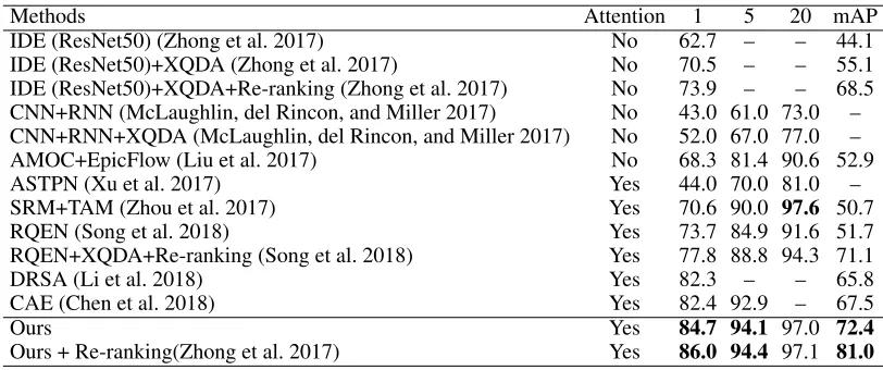
Table 3: Comparison with state-of-the-art methods on MARS in terms of CMC(%) and mAP(%). The methods using attention mechanism are indicated by ‘Attention’ column.
Methods Attention 1 5 20 mAP
IDE (ResNet50) (Zhong et al. 2017) No 62.7 – – 44.1 IDE (ResNet50)+XQDA (Zhong et al. 2017) No 70.5 – – 55.1 IDE (ResNet50)+XQDA+Re-ranking (Zhong et al. 2017) No 73.9 – – 68.5 CNN+RNN (McLaughlin, del Rincon, and Miller 2017) No 43.0 61.0 73.0 – CNN+RNN+XQDA (McLaughlin, del Rincon, and Miller 2017) No 52.0 67.0 77.0 – AMOC+EpicFlow (Liu et al. 2017) No 68.3 81.4 90.6 52.9
ASTPN (Xu et al. 2017) Yes 44.0 70.0 81.0 –
SRM+TAM (Zhou et al. 2017) Yes 70.6 90.0 97.6 50.7
RQEN (Song et al. 2018) Yes 73.7 84.9 91.6 51.7
RQEN+XQDA+Re-ranking (Song et al. 2018) Yes 77.8 88.8 94.3 71.1
DRSA (Li et al. 2018) Yes 82.3 – – 65.8
CAE (Chen et al. 2018) Yes 82.4 92.9 – 67.5
Ours Yes 84.7 94.1 97.0 72.4
Ours + Re-ranking(Zhong et al. 2017) Yes 86.0 94.4 97.1 81.0
Table 4: Comparison with state-of-the-art methods on LPW in terms of CMC (%). The methods using attention mecha-nism are indicated by ‘Attention’ column.
Methods Attention 1 5 20
GoogleNet(Song et al. 2018) No 41.5 66.7 86.2 RQEN(Song et al. 2018) Yes 57.1 81.3 91.5
Ours Yes 71.7 89.8 96.6
Video-based Person Re-identification
To further evaluate the effectiveness of our method, we con-duct experiments on video-based person re-identification
task.
Table 5: Ablation studies on CUB-200-2011, LPW, MARS in terms of Recall@K(%) and mAP (%).
CUB-200-2011 LPW MARS
K 1 2 4 8 16 32 1 5 20 1 5 20 mAP
GoogleNet 47.8 61.1 73.2 83.2 90.4 95.4 – – – – – – – Baseline 52.0 65.0 76.2 84.8 90.9 95.0 61.9 84.4 94.3 79.1 91.5 95.9 66.6 OSM 54.2 66.8 76.9 85.9 91.6 95.5 69.3 89.8 95.4 82.3 93.1 96.0 70.5 OSM+CAA 55.3 67.3 77.5 85.8 91.8 95.4 71.7 89.8 96.6 84.7 94.1 97.0 72.4
al. 2018), respectively. We report the Cumulated Matching Characteristics (CMC)2 results for both datasets. We also compute the mean average precision (mAP) for MARS. Comparative evaluation.The results of MARS and LPW are shown in Table 3 and Table 4 respectively. The results on both datasets demonstrate the effectiveness of our proposed approach. Our observations are as follows:
• On MARS dataset, our method outperforms all the meth-ods by a large margin. Compared with CAE (Chen et al. 2018)3, ours improves 2.3% and 4.9% in terms of CMC-1 and mAP respectively; When using re-ranking as post-processing in the test phase, the performance of our method further increases.
• On LPW dataset, we can see that our method again out-performs state-of-the-art methods by a large margin.
Ablation Study
Our key contributions in this paper are OSM and CAA. To evaluate the contribution of each module, we conduct abla-tion studies on CUB-200-2011, LPW, and MARS datasets. The details are as follows:
• Baseline: Neither OSM or CAA is used. Online pair con-struction is applied. The weight of each pair is fixed as one in the loss functions Eq. (7) and Eq. (8). Specifically,
w+ij= 1andwij−= 1.
• OSM: When mining negatives, OSM generates higher scores for difficult negatives and lower scores for trivial negative samples. When mining positives, OSM gener-ates higher scores for local positives to preserves intra-class variances. CAA is not used. Specifically,wij+ =s+ij
andw−ij =s−ij.
• OSM+CAA: As mentioned before, OSM is prone to out-liers similar to other mining methods, which is an inherent problem of mining approaches. Therefore, we combine OSM with CAA to conduct soft mining as well as address outliers. Specifically,w+ij=s+ij∗aijandwij−=s
− ij∗aij. The results are summarized in Table 5. We can see that OSM alone can achieve very competitive performance com-pared with the baseline. After integrating CCA to OSM, the accuracy increases on all datasets by about 1-2%. It is easy
2
CMC@Kis the same as Recall@K. Generally, the term CMC is used in person re-identification.
3
For CAE, we present the results of complete sequence instead of multiple snippets so that it can be compared with other methods. Multiple snippets can be regarded as data augmentation in the test phase.
to see that both OSM and CCA contribute positively toward the final performance.
Furthermore, we notice that test set classes of CUB-200-2011 overlaps with ImageNet (Russakovsky et al. 2015) dataset. To verify how much actually we improve, we show the performance of pre-trained GoogleNet (Ioffe and Szegedy 2015) without any fine-tuning. The result is shown in the first row of Table 5. Just using GoogleNet with pre-trained weights, the performance is 47.8% – already beat-ing most of the methods shown in Table 1. In contrast, our method outperforms pre-trained GoogleNet by a large mar-gin.
Conclusion
In this work, we propose a simple yet effective mining method named OSM. Importantly, OSM not only mines nontrivial sample pairs for accelerating convergence, but also learns extended manifolds for preserving intraclass variances. Besides, we propose CAA to address the impact of outliers. Finally, to evaluate the effectiveness of these two modules in action, we propose weighted contrastive loss by combining OSM and CAA to learn discriminative embed-dings. The experiments on fine-grained visual categorisation and video-based person re-identification with four datasets demonstrate the superiority of our method. For future work, it is interesting to see the integration of OSM and CAA for other kinds of losses such as triplet loss.
References
Bell, S., and Bala, K. 2015. Learning visual similarity for product design with convolutional neural networks. ACM Transactions on Graphics 98.
Chechik, G.; Sharma, V.; Shalit, U.; and Bengio, S. 2010. Large scale online learning of image similarity through ranking. The Journal of Machine Learning Research1109– 1135.
Chen, D.; Li, H.; Xiao, T.; Yi, S.; and Wang, X. 2018. Video person re-identification with competitive snippet-similarity aggregation and co-attentive snippet embedding. InCVPR. Cui, Y.; Zhou, F.; Lin, Y.; and Belongie, S. 2016. Fine-grained categorization and dataset bootstrapping using deep metric learning with humans in the loop. InCVPR.
Goldberger, J., and Ben-Reuven, E. 2017. Training deep neural-networks using a noise adaptation layer. ICLR. Hadsell, R.; Chopra, S.; and LeCun, Y. 2006. Dimensional-ity reduction by learning an invariant mapping. InCVPR. Harwood, B.; Kumar, B.; Carneiro, G.; Reid, I.; Drummond, T.; et al. 2017. Smart mining for deep metric learning. In
ICCV.
Hoffer, E., and Ailon, N. 2015. Deep metric learning using triplet network. In International Workshop on Similarity-Based Pattern Recognition.
Huang, C.; Change Loy, C.; and Tang, X. 2016. Unsuper-vised learning of discriminative attributes and visual repre-sentations. InCVPR.
Huang, C.; Loy, C. C.; and Tang, X. 2016. Local similarity-aware deep feature embedding. InNIPS.
Ioffe, S., and Szegedy, C. 2015. Batch normalization: Accel-erating deep network training by reducing internal covariate shift. InICML.
Jetley, S.; Lord, N. A.; Lee, N.; and Torr, P. H. 2018. Learn to pay attention.ICLR.
Jia, Y.; Shelhamer, E.; Donahue, J.; Karayev, S.; Long, J.; Girshick, R.; Guadarrama, S.; and Darrell, T. 2014. Caffe: Convolutional architecture for fast feature embedding. In
ACMMM.
Krause, J.; Stark, M.; Deng, J.; and Fei-Fei, L. 2013. 3d ob-ject representations for fine-grained categorization. InICCV Workshop.
Krizhevsky, A.; Sutskever, I.; and Hinton, G. E. 2012. Imagenet classification with deep convolutional neural net-works. InNIPS.
Li, S.; Bak, S.; Carr, P.; and Wang, X. 2018. Diversity reg-ularized spatiotemporal attention for video-based person re-identification. InCVPR.
Liu, H.; Jie, Z.; Jayashree, K.; Qi, M.; Jiang, J.; Yan, S.; and Feng, J. 2017. Video-based person re-identification with ac-cumulative motion context. IEEE Transactions on Circuits and Systems for Video Technology.
McLaughlin, N.; del Rincon, J. M.; and Miller, P. 2017. Video person re-identification for wide area tracking based on recurrent neural networks.IEEE Transactions on Circuits and Systems for Video Technology.
Oh Song, H.; Xiang, Y.; Jegelka, S.; and Savarese, S. 2016. Deep metric learning via lifted structured feature embed-ding. InCVPR.
Russakovsky, O.; Deng, J.; Su, H.; Krause, J.; Satheesh, S.; Ma, S.; Huang, Z.; Karpathy, A.; Khosla, A.; Bernstein, M.; et al. 2015. Imagenet large scale visual recognition chal-lenge.International Journal of Computer Vision211–252. Schroff, F.; Kalenichenko, D.; and Philbin, J. 2015. Facenet: A unified embedding for face recognition and clustering. In
CVPR.
Shi, H.; Yang, Y.; Zhu, X.; Liao, S.; Lei, Z.; Zheng, W.; and Li, S. Z. 2016. Embedding deep metric for person re-identification: A study against large variations. InECCV.
Simo-Serra, E.; Trulls, E.; Ferraz, L.; Kokkinos, I.; Fua, P.; and Moreno-Noguer, F. 2015. Discriminative learning of deep convolutional feature point descriptors. InICCV. Sohn, K. 2016. Improved deep metric learning with multi-class n-pair loss objective. InNIPS.
Song, G.; Leng, B.; Liu, Y.; Hetang, C.; and Cai, S. 2018. Region-based quality estimation network for large-scale per-son re-identification. InAAAI.
Sun, Y.; Chen, Y.; Wang, X.; and Tang, X. 2014. Deep learn-ing face representation by joint identification-verification. In
NIPS.
Szegedy, C.; Liu, W.; Jia, Y.; Sermanet, P.; Reed, S.; Anguelov, D.; Erhan, D.; Vanhoucke, V.; and Rabinovich, A. 2015. Going deeper with convolutions. InCVPR. Tadmor, O.; Rosenwein, T.; Shalev-Shwartz, S.; Wexler, Y.; and Shashua, A. 2016. Learning a metric embedding for face recognition using the multibatch method. InNIPS. Taigman, Y.; Yang, M.; Ranzato, M.; and Wolf, L. 2014. Deepface: Closing the gap to human-level performance in face verification. InCVPR.
Ustinova, E., and Lempitsky, V. 2016. Learning deep em-beddings with histogram loss. InNIPS.
Wah, C.; Branson, S.; Welinder, P.; Perona, P.; and Belongie, S. 2011. The caltech-ucsd birds-200-2011 dataset.
Wang, X., and Gupta, A. 2015. Unsupervised learning of visual representations using videos. InICCV.
Wang, J.; Song, Y.; Leung, T.; Rosenberg, C.; Wang, J.; Philbin, J.; Chen, B.; and Wu, Y. 2014. Learning fine-grained image similarity with deep ranking. InCVPR. Weinberger, K. Q., and Saul, L. K. 2009. Distance met-ric learning for large margin nearest neighbor classification.
The Journal of Machine Learning Research207–244. Xu, S.; Cheng, Y.; Gu, K.; Yang, Y.; Chang, S.; and Zhou, P. 2017. Jointly attentive spatial-temporal pooling networks for video-based person re-identification. InCVPR.
Yuan, Y.; Yang, K.; and Zhang, C. 2017. Hard-aware deeply cascaded embedding. InICCV.
Zhang, C.; Bengio, S.; Hardt, M.; Recht, B.; and Vinyals, O. 2017. Understanding deep learning requires rethinking generalization.
Zheng, L.; Bie, Z.; Sun, Y.; Wang, J.; Su, C.; Wang, S.; and Tian, Q. 2016. Mars: A video benchmark for large-scale person re-identification. InECCV.
Zhong, Z.; Zheng, L.; Cao, D.; and Li, S. 2017. Re-ranking person re-identification with k-reciprocal encoding. InCVPR.