Improving Variational Methods via Pairwise Linear
Response Identities
Jack Raymond [email protected]
Dipartimento di Fisica, La Sapienza University of Rome Piazzale Aldo Moro 5
Rome, Italy
Federico Ricci-Tersenghi [email protected] Dipartimento di Fisica, INFN–Sezione di Roma1 and CNR–Nanotec,
La Sapienza University of Rome Piazzale Aldo Moro 5
Rome, Italy
Editor:Manfred Opper
Abstract
Inference methods are often formulated as variational approximations: these approxima-tions allow easy evaluation of statistics by marginalization or linear response, but these estimates can be inconsistent. We show that by introducing constraints on covariance, one can ensure consistency of linear response with the variational parameters, and in so doing inference of marginal probability distributions is improved. For the Bethe approximation and its generalizations, improvements are achieved with simple choices of the constraints. The approximations are presented as variational frameworks; iterative procedures related to message passing are provided for finding the minima.
Keywords: variational inference, graphical models, message passing algorithms, statisti-cal physics, linear response
1. Introduction
Given a probability distributionp(x), estimation of marginal probability distributions such as p(xi) and p(xi;xj) is one of the most important inference tasks addressed in graphi-cal models, alongside estimation of the maximum probability state and the log partition function (see Wainwright and Jordan, 2008; Mezard and Montanari, 2009; MacKay, 2004). The challenge is addressed in many research fields by a variety of methods. In Boltz-mann machine learning and probabilistic independent component analysis the expectation-maximization algorithm requires such estimates (see Wainwright and Jordan, 2008; Miskin and MacKay, 2000). In heuristic optimization, a branch and bound search (or decimation procedure) over a high dimensional space can be made more efficient, by branching on xi (or some small set of variables) in an informed manner using approximate probabilities (see Montanari et al., 2007). In channel coding we wish to determine the likely state of a bit sent over a noisy channel, which can be inferred with a measure of certainty from the marginal probability (see Richardson and Urbanke, 2008). In statistical physics, marginal probability
c
distributions provide insight into phase transitions and thermodynamic phases (see Parisi, 1987).
Approximation of marginal probability distributions (called marginals henceforth) with high accuracy is NP-hard even in the case of Ising spins (binary variables) with pairwise interactions (see Dagum and Luby, 1993; Long and Servedio, 2010), but in practice, many schemes might be applied successfully. Approximate inference of marginal distributions is often performed by Markov chain Monte Carlo (MCMC) procedures (see Andrieu et al., 2003). These methods are a workhorse of inference, but have some disadvantages: the esti-mates are achieved with an accuracy that decays only slowly with time resources (exploiting the central limit theorem), the result is stochastic, and takes a non-parametric form. For these reasons variational approximations are often preferred, the price being a (difficult to quantify) bias in the approximations (see Wainwright and Jordan, 2008; Mezard and Montanari, 2009; MacKay, 2004).
In a basic variational approximation an intractable probability distribution p(x) is ap-proximated by a tractable one q(x), the parameters of q are determined by minimizing the Kullback Leibler (KL) divergence DKL[p||q]. The challenge of marginalization is thus replaced by two linked challenges: appropriate construction of q, and minimization of a KL-divergence. An example of a tractable distribution is a factorized one: q(x) =Q
iq(xi), which leads to a mean-field variational approximation; KL-divergence could then typically be minimized by an iteration of fixed point equations (see Wainwright and Jordan, 2008; Mezard and Montanari, 2009). It is common for the estimates obtained by variational ap-proximations to be over-confident, the uncertainty in some variables is reduced since the structure of the approximationq discounts some sources of variance.
A given variational framework may be minimized by several algorithms, and it is in-teresting that many famous heuristic algorithms developed independently of variational frameworks have been shown to be particular solutions to variational approximations. Most notably loopy belief propagation has been shown to be one method to solve the Bethe variational approximation, and expectation propagation was shown to be one method to solve the expectation consistent variational approximation. This connection to variational frameworks has allowed interesting insight into algorithm construction, proofs of solution existence and convergence (see Yedidia et al., 2005; Wainwright and Jordan, 2008; Yuille, 2002).
We will consider variational approximations applied to a model of N discrete variables
xi defined by probability 1
p(x) = 1
Z
M Y
a=1
ψa(xa), (1)
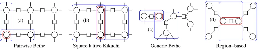
where ψa are the potentials (also called factors) and are non-negative functions of the variables indexed by subseta,xa={xi :i∈a},Z is the partition function. Probabilities of this kind can be represented as a factor graph (see Wainwright and Jordan, 2008; Mezard and Montanari, 2009), as shown in Figure 1. Our aim is to demonstrate a mechanism whereby existing variational schemes can be leveraged for improved inference of marginals. This paper considers a new self-consistent approximation to improve variational meth-ods, with an emphasis on the Bethe approximation and its generalizations (called region-based, or cluster-variational, approximations). We propose the addition of constraints re-quiring the consistency of estimates obtained via direct marginalization and linear response. We minimize the variational function subject to an agreement of these estimates and show that the resulting unique estimate is an improvement on the two estimates that are obtained without the constraints.
1.1 Literature Review
The linear response has been leveraged to improve estimates of marginals in a variety of problems, the idea originating in statistical physics (see Parisi, 1987; Opper and Winther, 2003; Welling and Teh, 2004).
Physics approaches often aim to improve understanding of phase transitions for problem classes in the limit of a large number of variables (see Parisi, 1987), rather than in develop-ment of algorithmic approaches to solve particular finite instances. An early application of linear response was the self-consistent Ornstein-Zernike approximation (SCOZA), proposed by Høye and Stell (1977), which was later applied by Dickman and Stell (1996) to simple graphical models. The SCOZA has been applied to disordered models where marginals are not homogeneous, for example to the random field Ising model in Kierlik, Rosinberg, and Tarjus (1999), but in the service of estimating globally averaged and disorder averages quantities, and never in such a way as to understand particular single variable or pairwise marginals, which is the question we address.
Opper and Winther (2001) proposed the adaptive-TAP approach as an extension of the standard Thouless-Anderson-Palmer mean-field method; in the original formulation of this method, a self-consistency relation between the linear response and magnetizations of a mean-field approximation were reconciled to arrive at a more advanced mean-field the-ory. Opper and Winther (2005) and Winther and Opper (2005) later reinterpreted this method as a special case of expectation consistent approximate inference, that made a con-nection between moment-matching algorithms such as expectation propagation and vari-ational frameworks, as well as expanding the range of applications. Expansions of the expectation consistent approximation to mitigate for errors on higher order cumulants have
shown promise in Opper, Paquet, and Winther (2013) and Paquet, Winther, and Opper (2009), but at this point come with few theoretical guarantees.
In the context of machine learning, other related approaches for improving mean-field estimation have been successfully demonstrated in Kappen and Rodriguez (1998) and Gior-dano, Broderick, and Jordan (2015). Mean-field variational Bayes is an important ap-plication of variational approximations, but the absence of an accurate understanding of covariance in the model parameters had been a weakness. Recently it was shown by Gior-dano, Broderick, and Jordan (2015) that linear response could be used to more accurately estimate these quantities.
The Bethe variational approximation is also an important approximation in the context of sparse graphical models, for which loopy belief propagation (LBP) is the most famous algorithm. Linear response has also been used to improve this approximation, examples in-clude Montanari and Rizzo (2005) and Mooij, Wemmenhove, Kappen, and Rizzo (2007). A large part of this development has been through loop-correction algorithms since the failure of the approximation is known to be related to loops in the graphical model representation. There also exist elegant loop correction methods not relying on the linear response: libDAI is a code repository that has collected some of the methods together (see Mooij, 2010), we developed our methods based on this library, in particular, the implementation of Heskes, Albers, and Kappen (2003). An expansion about the loop free approximation was developed by Chertkov and Chernyak (2006), but is cumbersome when many loops are present.
Several papers related to an extension of the Bethe approximation were published by Yasuda and Tanaka (2013), Raymond and Tersenghi (2013b),Raymond and Ricci-Tersenghi (2013a) and Yasuda (2013). The idea was very similar to that of adaptive-TAP, to minimize the variational function subject to the constraint of statistical consistency. When applied to the mean-field approximation it was realized these methods were equivalent to adaptive-TAP, but in the context of Bethe and region-based free energies improved perfor-mance was identified. In Raymond and Ricci-Tersenghi (2013b) and Huang and Kabashima (2013) linear response frameworks were also leveraged in the reverse direction to solve the inverse-Ising problem (inferring parameters from statistics).
These variational frameworks were applied initially to Bethe and mean-field approxima-tions on pairwise binary state models, in Yasuda (2013) an extension to general discrete states was provided, whereas Raymond and Ricci-Tersenghi (2013b) applied the technique to region-based variational frameworks and a broader range of constraint types. In this paper, we consider generic discrete alphabets, region-based free energies (inclusive of the Bethe ap-proximation) and both single-variable and pairwise variable consistency constraints. Build-ing on a belief propagation approach we derive tools for minimizBuild-ing constrained variational free energies.
1.2 Outline
Figure 1: The constrained variational approximations we present can be applied to models with multi-variable interactions, as represented by factor graphs. Two examples are shown. Top: the alarm network is a well-known toy example of a Bayesian net, here represented as a factor graph. Squares denote factors ψa(xa), which act over subsets of variables xa, each variable represented by a circle. Bottom: N = 10 variables interacting according to a random cubic graph is represented, each coupling (J) is represented by a factor with two connections, each field (h) by a singly connected factor.
and other insights gained, before concluding in Section 6. Appendices include exact ex-pressions for the fully connected ferromagnet example, pseudocode and algorithmic details, proofs of convergence for some methods, discussion of solution existence and convergence, and how to select constraints for inclusion.
2. Constrained Variational Approximations
Variational free energy approximations are powerful tools for approximate inference (see Yedidia et al., 2005; Opper and Winther, 2005; Wainwright and Jordan, 2008; Mezard and Montanari, 2009). We introduce in this section the mean-field, Bethe, and region-based (also called Kikuchi) approximations. A set of simplified expressions appropriate to the Bethe approximation for an Ising model is given alongside the general expressions. We first introduce a generalization of the probability over the N variables x, introducing auxiliary parameters ν,
pν(x) = 1
Z(ν) M Y
a=1 ψa(xa)
N Y
i=1
"
Y
y
exp (νi,yδxi,y) #
. (2)
This coincides with (1) in the limit ν → 0. The product on y is over all possible states of xi. For our method to apply the probability needs to be differentiable with respect to the parameters ν, though modifications allow for the more general case2. The choice of statistics {δxi,y} simplifies our presentation, but more generally we might consider a set of single variable functions{φy(xi)}, this is discussed in Appendix B.2.
A Boltzmann machine will be presented as a running example. The model3 has Ising spin variablesx∈ {−1,1}N, fieldshand pairwise couplingsJ. A connected graphical model will be assumed for notational simplicity, so each variable has connectivity ki ≥ 1, and a unique connected component exists. If an edge set E = {(i, j)} specifies the interacting
2. Special care should be taken in cases where ψa(xa) = 0 for some xa, in such cases it may not be meaningful to perturb by ν. Furthermore, we note that ν are a redundant set of parameters since variation ofP
yνi,yleaves the probability unchanged.
variables, then
pν(x) = 1
Z(ν)
Y
(i,j)∈E
exp(Jijxixj) Y
i
exp[(hi+νi)xi], (3)
where we use a non-redundant set of auxiliary parametersνi =νi,1−νi,−1.
In a variational approximation a trial probability distribution q(x) is related to the log-partition function of the full model, derived from the Kullback-Leibler divergence
DKL[q||pν] = X
x
q(x)
logq(x)− X
i,y
νi,yδxi,y− X
a
logψa(xa)
+ logZ(ν). (4)
The variational free energy (VFE) is defined
Fν(q) =DKL[q||pν]−logZ(ν), (5)
which is the tractable part of (4). The optimal variational parameters q∗ are those mini-mizing (5).
In the simplest mean-field approximation a factorized variational form is considered
q(x) = QN
i=1qi(xi). The parameters {qi} are precisely marginal distributions on single
variables. Iterative methods are often successful in minimizing the VFE. In another class of approximations the entropy term in the VFE, −P
xq(x) logq(x), is decomposed as a truncated sum of marginal entropies. In the Bethe approximation a redun-dant set of marginal probability distributions{qa(xa);qi(xi)}4 are introduced in one-to-one correspondence with the model factors and variables, and the entropy is approximated as
−X
x
q(x) logq(x)≈ −X a
X
xa
qa(xa) logqa(xa)− X
i
(1−ki) X
xi
qi(xi) logqi(xi), (6)
withki equal to the variable connectivity (the number of factors in which variablei partici-pates). The reason this approximation may improve upon mean-field is that throughqa(xa) some correlations amongst variables may be explicitely represented, which are absent in the factorial form of mean-field. The variational parameters, qa and qi, are referred to as beliefs.
The Bethe approximation is a special case of the more general region-based approxima-tion (see Yedidia et al., 2005), where the entropy approximaapproxima-tion is implied by a choice of outer regions. Each outer region is defined by a set of variablesxα, and a generalized factor
ψα(xα) that describes the interactions between those variables. The outer regions must be chosen to span all variables, and the factors (as well as auxiliary parametersν) can be distributed amongst the generalized factors such that Q
αψα(x) ∝pν(x). Some examples of region selections discussed in this paper are shown in Figure 2.
The entropy approximation is implied by the choice of outer regions: it is the sum of the entropy on the outer regions α corrected by a weighted sum of entropies on region
(d)
(c)
Square lattice Kikuchi (b)
(a)
Generic Bethe Region−based
Pairwise Bethe
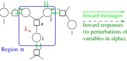
Figure 2: In a region-based approximation (Bethe is a special case), the assignment of outer regions determines the entropy approximation. Sensible choices collect nearby sets of strongly dependent variables. A region graph has outer regions (blue) and intersection regions (red), such that every factor is associated to exactly one outer region; the set of factors in a region α define an auxiliary interaction (8). Selection (a) is a Bethe approx-imation, the outer regions are pairs of variables, that intersect on single variables. (b) Alternatively, for a square lattice, we might consider outer regions of 4 variables (the cen-tral interaction could be assigned to either the right or left region), that intersect on pairs of variables, which in turn intersect on single variables. This approximation is powerful for square lattice models (see Raymond and Ricci-Tersenghi, 2013b; Dom´ınguez et al., 2011; Lage-Castellanos et al., 2013). (c) The Bethe approximation on a factor graph with mixed (multi-variable) interaction types has outer regions containing exactly one factor and its variables, the intersections are single variables. (d) On a locally tree-like graph, we can also make an interesting approximation: outer regions are stars that intersect on edge regions. This approximation relates to the loop-correction algorithm of Montanari and Rizzo (2005).
intersections (β). The region based free energy is defined
Fν(q) = X
α X
xα
qα(xα) log
qα(xα)
ψα(xα)
+X
β
cβ X
xβ
qβ(xβ) logqβ(xβ), (7)
where cβ take integer values according to a simple rule (see Yedidia et al., 2005; Heskes et al., 2003). Larger regions are capable of capturing more correlations between variables explicitely, but at a computational cost that scales (in the absence of further approxima-tions) exponentially with region size. This trade-off determines the choice of regions.
In the Bethe approximation, the outer regions (α) are in one-to-one correspondence with the factors (a) of the model, and intersection regions are single variables. In our running example of the Boltzmann machine (3), a Bethe approximation has edges as regions. Generalized factors can be chosen as
ψ(i,j)(xi, xj) = exp
Jijxixj +
hi+νi
ki
+hj +νj
kj
. (8)
We can define marginal variational parameters for each marginal probability in the free energy and then minimize (7) subject to local consistency constraints
X
xα
qα(xα) = 1 ; ∀α , (9)
X
xα\xβ
Minimization of this free energy is a well-studied problem. Heuristic approaches normally lead to message passing algorithms, which are often convergent to good solutions even where guarantees of convergence are lacking. It is always possible to find minima of the region based free energy using a convex-concave procedure, which is guaranteed to converge to a local minima (see Yuille, 2002; Heskes et al., 2003).
Having found a minimum of the free energy atq =q∗, we can define the linear response in the beliefs to a perturbation inνi,y, as
qα,∗(i,y)(xα) =
∂qα(xα)
∂νi,y
q=q∗
.
Whereas the variational parametersqhave an interpretation away from the fixed point, the linear response is only defined about a global (or heuristically, local) minima. Notation ∗ will be used to denote an evaluation at such a fixed point.
The entropy approximations (6-7) can be interpreted as truncated series (see Pelizzola, 2005; Wainwright and Jordan, 2008), that can be made good either by considering suffi-ciently large regions (those defining a junction tree, see Wainwright and Jordan, 2008), or including loop corrections (see Chertkov and Chernyak, 2006). The made-good approaches are not tractable in many interesting models of modest scale. The region based methods most often lead to improvements over mean-field, but entropy expansion can also lead to counterintuitive features. For example, the entropy estimate can be negative under such an approximation.
2.1 Inconsistency of Covariance Approximations
The covariance of a pair of statisticsφ1 andφ2, under probability distribution p is defined
as
Vp(φ1, φ2) = Ep(φ1φ2)−Ep(φ1)Ep(φ2),
with Ep(φ) = X
x
p(x)φ(x).
For the caseφ1(xα) =δxi1,y1 andφ2(xα) =δxi2,y2, we can replace the probability of interest
p byqα to obtain
Vp(δxi1,y1, δxi2,y2)≈C(i1,y1),(i2,y2):=Vqα[δxi1,y1, δxi2,y2].
C will be called the marginal approximation to the covariance, and is a function of the variational parameter qα. The optimal value C∗ = C(q∗) is independent of the region α, owing to the consistency constraints (9)-(10).
Alternatively, we can begin with a second derivative identity. By introducing parameters
ν conjugate to each statistics (2), we have
Vp(δxi1,y1, δxi2,y2) =
∂2logZ(ν)
∂νi1,y1∂νi2,y2
.
We obtain a tractable approximation replacing logZ(ν) by−Fν(q∗)
Vp(δxi1,y1, δxi2,y2)≈χ(i1,y1),(i2,y2):=
X
xα
for any α containing i2, which is called the linear response estimate. χ will be called the
linear response approximation to the covariance, it is defined only at the minima q∗, and is a symmetric matrix. We do not need to make explicit reference to the region α used in Eq. (11) since the linear responseχ does not depend on that choice.
The name ‘linear response’ for the quantity χcomes from the fact it can be interpreted as
χ(i1,y1),(i2,y2)≈
∂Ep[δxi1,y1]
∂νi2,y2
ν=0
= ∂Ep[δxi2,y2]
∂νi1,y1
ν=0
, (12)
that is the linear variation of the mean value of a single variable statistic to a small pertur-bation in the the parameter ν conjugated to another single variable statistic.
We denote the difference of these estimates for two statistics on variables (i1, i2)
con-tained in regionα as
∆(i1,y1),(i2,y2),α(qα, q∗α,(i1,y1)) =C(i1,y1),(i2,y2)−χ(i1,y1),(i2,y2) . (13)
Except for some simple modelsC∗−χ is non-zero, exposing an inconsistency in the varia-tional method. The best marginal approximation does not match the best linear response estimate. To decide which estimate to use, either connected correlations or linear responses, we might consider the distance of these two different estimates from the correct value:
∆(1)(i1,y1),(i2,y2) = C(∗i1,y1),(i2,y2)−Vpδxi1,y1, δxi2,y2
, (14)
∆(2)(i1,y1),(i2,y2) = χ(i1,y1),(i2,y2)−Vpδxi1,y1, δxi2,y2
. (15)
Graphical models in which the Bethe approximation is most successful have relatively weak correlations and/or few short loops. In these cases it is known that the linear response estimate (15) improves significantly upon (14) for i1 6= i2 (see Welling and Teh, 2004;
Raymond and Ricci-Tersenghi, 2013a). However, as the approximation breaks down (due to poor approximations of loops in the graphical model), the response estimate can be much worse, even giving infinite values for bounded statistics. For pairs withi1 =i2 (called
diagonal), bounds can be violated even in regimes where the approximation is good. A simple example is the model of Section 4.1 with zero field (h = 0): whilst it is true that
Vp(xi, xi)≤1 for any model,χi,i >1 for in the weakly coupled (high temperature) regime.
2.2 Covariance Constraints
We would like to use the linear response information, in a safe manner to select the best covariance estimate, but also to make the approximation self-consistent. Rather than simply minimizing the free energy to determine q∗, we do this in the subspace where {∆(i1,y1),(i2,y2),α= 0}for a subset of the covariances.
An important question will be which covariances to constrain. Expansion methods indi-cate that adding all constraints is best when the approximation is very good (see Raymond and Ricci-Tersenghi, 2013a). More generally we wish to add important constraints in so far as it does not prevent solution existence and allows algorithmic stability as discussed in Appendices B.1-B.3.
discussed in Appendix B.2. The Bethe approximation with the addition of all possible con-straints (calledon and off diagonal5) is considered, as well as the Bethe approximation with addition of only constraints for whichi1 =i2 (diagonal). In Section 4.1 we also present
re-sults for the mean-field approximation with all possible constraints (sincei1 =i2in all cases,
this is also called diagonal), as well as the Bethe approximation including only constraints for which i1 6= i2 (off-diagonal). In other experiments, we do not present these latter two
regimes since they performed consistently worse except in some narrow parameter ranges where all regimes were performing poorly.
2.3 Bethe Approximation to the Boltzmann Machine
In the case of our running example of the Boltzmann machine (3) we are considering a variation ofνi =νi,1−νi,−1, accordingly we can abbreviate notation everywhere (i, y) to i.
In the diagonal constraint approximations, we will require consistency of V(xi, xi) ∀ i. In the on and off diagonal constrained approximations, we require in addition consistency of V(xi, xj) for all coupled pairs of variables.
The quantities made consistent are written more concisely as
Vp(xi, xj) ≈ Ci,j :=Vq(ij)(xi, xj),
Vp(xi, xj) ≈ χi,j := X
xi,xj
q(∗ij),i(xi, xj)xj .
When evaluated at minima of the free energy, both the approximation by marginalization
C∗, and approximation by linear responseχ, are symmetric.
3. Minimizing with Respect to the Constraints
We choose a Lagrangian formulation for minimizing the constrained free energy, introducing a Lagrange multiplier for each constraint connecting a linear response approximation to a marginalization approximation. Each statistic pair constraint will be associated with some unique outer region α, as this allows for a cavity heuristic that we later introduce. This association is not unique and may affect (to a limited extent) the convergence of the algorithms we will develop, but not the fixed points that might be achieved. This is discussed further in Appendix B.3. The set of constraints associated to regionαare denoted
ωα ={[(i1, y1),(i2, y2)]}with an associated set of Lagrange multipliersλα={λ(i1,y1),(i2,y2)}.
The constrained minimization is then achieved by minimizing the Lagrangian
Fν(q, λ, χ) =Fν(q)+ X
α
X
[(i1,y1),(i2,y2)]∈ωα
λ(i1,y1),(i2,y2)∆α,(i1,y1),(i2,y2)(qα, q∗α,(i1,y1))
, (16)
with Lagrange multipliers set to meet the constraints. The global minimaq∗ for fixedλcan often be found. In cases where local minima can be avoided this is done either heuristically following a constrained loopy belief propagation (CLBP) approach, or in a more robust manner using a provably convergent method, as discussed in Appendix B. CLBP has the same (asymptotic) computational complexity as belief propagation, and is procedurally similar.
Compute the minima q* of the free energy F(q,
Compute Lagrange multipliers by solving {C* = } on outer regionsχ
λ Compute the linear responses χ
λ,χ)
Figure 3: The basic scheme for minimizing our constrained variational free energy. The first stage is solved by a procedure closely related to belief propagation (that minimizes a convex-concave function), the second by a procedure related to susceptibility propagation (that solves a system of linear equations), and the final stage by a cavity approximation. In our experiments, we take λ= 0 as the initial condition. In the experiments presented we gradually increase or decreaseT using the solution atT±δT as an initial condition for the next experiment, this enables a solution to evolve continuously from a well-understood limit, but is not necessary for convergence in general.
It is shown in Appendix B.6 that given such a fixed point, whether a local or global mini-mum, it is subsequently relatively easy to calculate the linear response. The method we pro-pose is procedurally similar to susceptibility propagation, originally introduced in Mezard and Mora (2008), which is a computational procedure that minimizes the variational pa-rameters. If the number of constraints is linear in the size of the system the computational complexity is quadratic in system size. We call the linear response scheme constrained loopy susceptibility propagation (CLSP). Yasuda and Tanaka (2013) proposed a closely related approach, specific to the case of diagonal constraints in the Bethe approximation.
Suppose we also have a method for iteratively determiningλ, then we can approach the problem of finding a constrained local minima by a 3-stage iterative procedure (the same as proposed in Yasuda and Tanaka (2013)), and shown schematically in Figure 3. We also experimented with other minimization schemes, but found this to be algorithmically the most stable, and also pleasing in that we move all uncertainty in convergence of the method onto the two questions: (1) does there exist a fixed point at all and (2) does the iterative scheme for λ converge. These two questions are unfortunately very difficult to answer in general. To determineλa heuristiccavity method is proposed in Section 3.1.
3.0.1 Bethe Approximation to the Boltzmann Machine
For the on-and-off diagonal constrained case, the Lagrangian for the Boltzmann machine can be written in the form6.
Fν(q,λ, χ) = X
(i,j)∈E X
xi,xj
qij(xi, xj) logqij(xi, xj) + X
i
(1−ki) X
xi
qi(xi) logqi(xi)
+1 2 X i λi,i
(1−Mi2)−χi,i
+ X
(i,j)∈E
λ(i,j)
X
xi,xj
qij(xi, xj)xixj−MiMj−χi,j
, (17)
introducing abbreviations for single variable magnetizationMi :=Pxiqi(xi)xi. We recover the diagonal constraint regime whenλi,j = 0 ∀i, j, and the unconstrained regime when all multipliers are zero. Constraints introduce quadratic functions ofq, but terms are neither convex nor concave.
For given λ, a set of message passing equations can be written as a generalization of loopy belief propagation, a simplification of the general case in Appendix B.5 is presented here. At time tthe edge-belief is approximated as the solution to the equation
qijt(xi, xj)∝µti→(i,j)(xi)µtj→(i,j)(xj) exp
(Jij−λij)xixj+ (hi+λijMij,jt +λiMij,it )xi+ (hj+λijMij,it +λjMij,jt )xj
,
where we introduce two auxiliary magnetization parameters per edge7 Mij,it =X
xixj
xiqijt(xi, xj). (18)
Then we can define messages8 µwhich are determined iteratively as µt(i,j)→i(xi) ∝
X
xj
µtj→(i,j)(xj) exp
(Jij−λij)xixj+ (hj+λjMij,jt +λijMij,it )xj+λijMij,jt xi
,
µti+1→(i,j)(xi) = Y
k∈∂i\j
µt(i,k)→i(xi), (19)
where ∂i are the variables interacting with i. Following message updates qt and Mt must be made consistent, in the examples of this paper (and in general for small λ) this can be achieved simply by iterating Equations (18) and (19). For the experiments messages and beliefs are initialized as constants.
There are several methods by which linear response can be established. One standard approach is susceptibility propagation, which simply involves linearizing the above equations accounting for a small perturbation in some component ofν, this is the approach taken for the examples of this paper; for the general case, expressions are provided in Appendix B.6.
6. To maintain consistency with published research on Ising spin models a factor 1/2 precedes the diagonal constraint term.
7. Note that at intermediate stages of the message passing, magnetizations for variableion different beliefs (sayMij,i,Mik,i) may not agree, but will agree after convergence.
λα Inward responses (to perturbations of variables in alpha). Inward messages
a
i j
Regionα
Figure 4: GivenC∗ andχ, determination ofλbreaks into a set of independent problems on outer regions α. This can be understood as a cavity approximation. Assuming the incom-ing messages, and responses, to be fixed and approximately independent of the Lagrange multipliers to be set (λα), we can independently, on each region, solve the system of equa-tions∆α = 0 for λα. A similar assumption often justifies message passing and mean-field iterative heuristics.
3.1 Determination of λ
To determine λwe propose the following scheme. We wish to solve at eachα a set of non-linear equations{∆α(qα, q∗α,(·)) = 0}, whereqαand q
∗
α,(·) are functions of allλ(through the
system of message passing equations). One possibility is to linearize these equations about the current estimate (that is apply Newton’s method), but this leads to an impractical
O(N3) procedure, dominating other algorithmic time-scales for moderately sized systems. Instead, we resort to a locally consistent and parallelizable approximation: For some
λ we find a minimum defined by messages µ (Appendix B.5), and the linear response for these messages (Appendix B.6). If λ is approximately correct then the messages passing into the region α should be weakly dependent on any changes to λα in that region. Since we can define∆α in terms of the local parametersλα, and the incoming messages (which we argue are unchanged by an update ofλα) the problem for determining λ is reduced to solving forλα independently on every region.
In this way, we arrive at a cavity-approximation style argument common in the moti-vation of message passing algorithms, see Figure 4. However, it is noteworthy that unlike LBP, incoming messages and responses depend on λα locally. There is a direct feedback that exists even in the absence of loops.
Unfortunately,∆α=0remains a (small) system of non-linear equations inλα, that does not allow a closed form solution in general. One exception is when only diagonal constraints are applied (see Yasuda, 2013; Yasuda and Tanaka, 2013), and the cavity argument is applied to single-variable regions. More generally we use Newton’s method to solve these equations
"
∂∆α(q∗, q(∗·))
∂λα
#−1
∆α
λ=λt
δλtα+1 =−∆α(q∗, q∗(·))
λ=λt , (20)
4. Results
In this section, we study the performance of our method on well-understood toy model frameworks. The scale and/or symmetries of these models mean they are exactly solvable, allowing precise statistical estimates to evaluate the method quality.
In Section 4.1 we study a fully connected ferromagnetic model (that is a model with a positive coupling between any pair of variables) with symmetry broken (that is with a non-zero mean value for each variable). This is a simple model for which we can present analytic results and understanding. There is either no mode (for weak coupling), or one dominating mode (for strong couplings). We expect the method to be weakest for intermediate coupling strength since the Bethe approximation becomes exact (with corrections O(1/N)) in the limit of strong (a single mode) or weak (no modes) coupling. In Section 4.2 we study a model with frustration (that is couplings have different signs and it is not possible to find a configuration satisfying them all at the same time) and a random distribution of optima and sub-optima. The problem is multi-modal in the limit of strong couplings and the Bethe approximation breaks down. In Section 4.3 we consider a simple model with an expanded discrete alphabet, where randomness is introduced through a random graphical structure. Like the ferromagnetic example, a single mode dominates for strong couplings. We anticipate the Bethe approximation to become exact in the limit of large problems, but for smaller problems the presence of short loops leads to inaccuracy. In the final example of Section 4.4 we consider a well-studied toy model involving both multi-variable interactions and multi-states, both the Bethe approximation and linear response perform poorly on this model. These examples cover a range of scenarios in which our method might be applied. Special cases of the variational approximation we present have previously been applied to lattice models commonly studied in statistical physics, and sparse prior models in Bayesian image modeling (see Raymond and Ricci-Tersenghi, 2013b,a; Yasuda and Tanaka, 2013; Yasuda, 2013).
We present behaviour of the Lagrange multipliers λ, the self-consistency error (13), errors on the pair statistics when using either marginals (14) or linear responses (15), and errors on the marginal estimates
∆(0)(i,y)(q∗) =q∗(xi =y)−p(xi =y).
The maximum absolute deviation (MAD) on the marginals is defined as the largest error over all variables, or pairs of variables, depending on error type.
It is interesting to understand how the quality of approximation changes as a function of the goodness of the approximation, to do this we introduce a temperature parameterT
in each model, that can sharpen or flatten the distribution.
pT(x)∝p(x)1/T .
We can minimize with relative ease both the constrained and unconstrained free ener-gies in the large T regime, and expect approximations to be correct at leading order in 1/T (see Raymond and Ricci-Tersenghi, 2013a). In some cases of small T, in which the probability is well described by a single mode, concentrated about some unique value
We find that in many of the models, minimization of the constrained free energy is slow or impossible for T over some intermediate range, or below some threshold. To extend the range ofT for which solutions could be found, an annealing procedure is employed: begin-ning at large (or small) T and proceeding through a sequence of models slowly changing
T, and using the solution to the previous model as the initial condition for the subsequent minimization. Under this procedure, we find that λ(T) and the variational parameters q
evolve smoothly, but that there appears still to be a limit in the accessible temperature range. In the applications presented we did not find fixed points that appeared discontin-uously. Solutions are reached by annealing from low temperature, from high temperature, or are absent.
Our motivation for introducing T is threefold: to study the breakdown of the approx-imation (absence of solutions), to mitigate for non-convergence, and to increase the speed of convergence. The annealing procedure introduces additional computational costs. We have not made timing comparisons against loopy belief propagation or other competitors, for either the simple or annealed procedure. Instead, we have prioritized an exploration of the nature of solutions that can be discovered, and we have sought very accurate estimates to the parameters describing those solutions. Compromises in the accuracy of constraint satisfaction, annealing rate (or absence of annealing), and damping can all have a significant impact on the speed of the method.
4.1 The Fully Connected Ferromagnet
We begin with a simple but informative case, that of a fully connected ferromagnetic Ising model in an external field.
pT(x) = 1
Z exp
1
2T h+
N X
i=1 xi
!2
. (21)
Variables are Ising spinsxi =±1. The marginals for this model can be solved up toO(1/N) by the mean-field approximation, and up toO(1/N2) by the Bethe approximation. Accuracy
is a function of temperature; when this is large or small compared to 1/N, the accuracy is correspondingly high. Under our method the equations to be solved and associated errors can be expressed concisely; this is done in Appendix A.
Three kinds of constraint are considered: diagonal {∆ii = 0, ∀ i}; off-diagonal{∆ij = 0, ∀i 6= j}; and on-and-off diagonal applying both sets. Results for both the mean-field and Bethe approximations are presented. Only diagonal constraints can be applied in the mean-field case since the variational parameters are consistent only with zero off-diagonal covariances.
0 0.05 0.1 0.15 0.2 0.25 0.3 0.35 0
0.1 0.2 0.3 0.4 0.5 0.6 0.7 0.8 0.9 1
Inverse Temperature, 1/T
Magnetization, E[x
i
]
Exact Mean Field Bethe MF: On Bethe: On Bethe: Off Bethe (On−and−off)
0 0.05 0.1 0.15 0.2 0.25 0.3 0.35
−0.25 −0.2 −0.15 −0.1 −0.05 0 0.05 0.1 0.15 0.2
Inverse Temperature, 1/T
Lagrange multiplier,
λ
λ
0
λ
1 MF: On Bethe: On Bethe: Off Bethe (On−and−off)
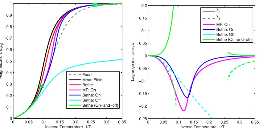
Figure 5: Results for the fully connected model (21) with N = 10 and h = 1. Re-sults are presented for the mean-field and Bethe approximation schemes, with and without constraints. (left) The magnetization is overestimated in the Bethe and Mean-field approx-imations, the effect of the constraints is to suppress the magnetization. Certain solutions exist only in the high-temperature or low-temperature regimes, those solutions are demar-cated by ’x’. One solution to the Bethe approximation with off-diagonal constraints only suppresses the magnetization too strongly, there is another solution that is present only at low temperature, where the estimate is more reasonable. Where it exists, the Bethe approx-imation with on and off-diagonal constraints is the most accurate. (right) There are at most two independent values forλin this model: diagonalλ0 and off-diagonalλ1. The Lagrange
In some constrained approximations there is a smooth evolution of the optimal beliefs with T, which reflects the behavior of the exact marginals. In others, the optimal beliefs for different T are not continuously related.
When off-diagonal constraints are applied in the Bethe approximation, either alongside or without diagonal constraints, we see a discontinuous emergence of the strongly magne-tized solution. In the case of only off-diagonal constraints, there is a coexistence of two fixed points for smallT. This means that as we vary the parameterT theq∗ moves discon-tinuously from a relatively smooth approximation to one characterized by a single mode. As N increases the domain with coexistence shrinks, and all approximation approach the correct result for largeN.
With on and off-diagonal constraints we find a range of T for which no solutions can be found by a continuous evolution of the low or high-temperature solutions. It seems highly likely that no solution exists, and empirically we were not able to find fixed points (for any model) that were not continuously related to either a high or low-temperature solution.
The behaviour of λ (see right panel in Figure 5) and indeed a careful examination of the fixed points indicate why solutions disappear in this simple case. The values of the Lagrange multipliers diverge, and this is related to marginals approaching their boundary values where variational inference breaks down due to the inflexibility of the parameters. By decreasinghorN we decrease the accuracy of the Bethe approximation at intermediate
T, this can lead to discontinuity also for the diagonal constrained solution, and reduces the range of temperatures over which the low-temperature solution (the one with a large magnetization) can be found for constrained problems.
4.2 The Wainwright-Jordan Set-up
A common toy model on spin variables xi = ±1 is the Wainwright-Jordan set-up where
N =L×LIsing spins are arranged on a square grid (see Opper et al., 2009).
pT(x) = Y
(i,j)∈E
exp(Jijxixj/T) Y
i
exp(hixi/T).
Fields hi are independent and identically distributed (iid) samples from [−0.25,0.25] and couplings Jij are sampled i.i.d on [−1,1]. The Bethe approximation fails on these models for smaller T owing to multi-modality of the distribution, but for larger T (where corre-lations are weaker) the approximation is a significant improvement upon the mean-field approximation.
Diagonal {∆i,i = 0, ∀i}, or diagonal and off-diagonal {∆i,j = 0,∀(i, j)∈E}constraint regimes are studied for the Bethe approximation.
is CLBP with on and off-diagonal constraints. The exact range of T for which methods were convergent was sensitive to the annealing procedure, the amount of damping used, and the convergence criteria; strong damping and slow annealing broaden the range for all methods.
Where the algorithm is convergent, there is significant improvement adding diagonal constraints, and more so with on and off-diagonal constraints.We find the improvement in the maximum deviation represents well the changes seen across the entire distribution of marginals in most models, almost all marginals are improved. The quartiles in figures 6 and 7 reflect model to model variations, and demonstrate that the MAD advantage is robust. ForN = 16, we can compare the median behavior against that reported in Opper, Paquet, and Winther (2009); where the strongest method (tree-EP) also improves the MAD result for marginals by approximately one order of magnitude. Expansion methods offer some further, but modest gains (see Paquet et al., 2009; Opper et al., 2013).
On-diagonal constraints allow an increased range (inT) for convergence. Qualitatively, we offer the following explanation. In the constrained regimes (in the high-temperature regime, the only one for which we demonstrate solutions) the majority of Lagrange multipli-ers are negative. The effect is to suppress biases and decrease susceptibility (the sensitivity of biases to small changes in the parameters). We assume that reduced susceptibility also correlates with reduced sensitivity to small fluctuations in the messages, which should aid algorithmic stability. With on-and-off diagonal constraints the diagonal and off-diagonal Lagrange multipliers are strongly dependent where they constrain the same variable. The off-diagonal multipliers are typically negative, and suppressing biases; by contrast, the diag-onal multipliers are positive and reinforce biases. The typical net effect is to reduce biases and susceptibility, as with the on-diagonal case. However, the strongly correlated nature of the parameters may be the source of convergence problems.
The failure of CLBP is most often due to non-convergence of λ, rather than a failure in the CLBP or CLSP iterative algorithms (at fixed λ). Figure 8 indicates why the iterative update is failing: some Lagrange multipliers are diverging in a strongly correlated manner and it seems likely there is a critical value of T close to the failure point beyond which no solutions exist, as found in Section 4.1.
The LBP implementation follows the same procedure as the constrained cases of Ap-pendix B, with the difference that the innermost do-while loop is always convergent in one iteration, and λ = 0. Using a double loop procedure we might force convergence to a minimum of the Bethe approximation, but the convergence properties of LBP are still an interesting point of comparison.
We might seek to extend the range of convergence for CLBP by clever modifications. However, it seems that breakdown of convergence is closely related to breakdown of the underlying (Bethe) approximation. Algorithmic innovations would not extend significantly the range of problems for which the constrained approximation is useful in practice; just as the availability of double loop methods has not revolutionized the use of the Bethe approx-imation: where LBP fails the Bethe approximation is almost always a poor approximation.
0.2 0.3 0.4 0.5 0.6 0.7 0.8 0.9 1
10−4
10−3
10−2
10−1
Model rescaling, 1/T
MAD for marginals, max(|
∆
(0
)|)
No constraints Diagonal constraints On−and−off diag. cons. Median
Lower Quartile Upper Quartile
0.3 0.4 0.5 0.6 0.7 0.8 0.9 1 10−4
10−3 10−2 10−1
Model rescaling, 1/T
MAD for pair connected correlations
No constraints Diagonal constraints On−and−off diag. cons. Median MAD C
ij: max(|∆ (1)|)
Median MAD χ ij: max(|∆
(2)|)
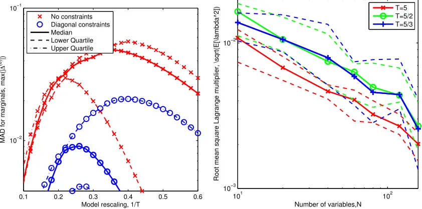
Figure 6: L= 4 Wainwright-Jordan set-up: The error on the marginals, and connected cor-relations (which together provide a sufficient description of pair probabilities) are improved everywhere by adding constraints, as long as the method converges. As discussed, the MAD forCij is worse than for χij, although they are becoming comparable approaching T = 1. On the right the median over 20 models is shown, on the left the median and quartiles. The advantage is consistent across all models.
Kikuchi approximations also indicate a modest decrease in error on marginals with the application of constraints.
4.3 Potts Model in an External Field
Next we consider random 3-regular graphs G= {V, E} of N = |V| variables, where each variable is allowed 3 states: xi ∈ {0,1,2}. The problems are defined by the probability
p(x)∝ Y
(ij)∈E
exp Jijδxi,xj/T Y
i∈V
exp (4δxi,0/T) ,
where couplings are i.i.d. random variables Jij ∈ {−1,1}. An example of a corresponding factor graph is shown in Figure 1 (lower panel). Like the fully connected Ising model, typical instances of this model are solved at leading in order in N by the Bethe approximation, with finite size effects strongest at intermediate temperatures. At high temperature, the probability is relatively flat and disperse, whereas at low temperatures there is a single dominating mode concentrated about the value 0= argmaxxp(x).
We consider a diagonal constrained Bethe approximation: a set of 4 non-redundant statistic pairs are constrained per variable.
0.2 0.3 0.4 0.5 0.6 0.7 0.8 0.9 1
10−4
10−3
10−2
10−1
Model rescaling, 1/T
MAD for marginals, max(|
∆
(0
)|)
No constraints Diagonal constraints On−and−off diag. cons. Median
Lower Quartile Upper Quartile
0.2 0.3 0.4 0.5 0.6 0.7 0.8 0.9 1 10−4
10−3 10−2 10−1
Model rescaling, 1/T
MAD for pair connected correlations
No constraints Diagonal constraints On−and−off diag. cons. Median MAD Cij: max(|∆(1)|)
Median MAD χ ij: max(|∆
(2)
|)
Figure 7: L= 7 Wainwright-Jordan set up: Trends are comparable to the smaller system in Figure 6. Where solutions exist, significant gains are made in all models with the addition of constraints. However, all approximations are now failing to reach full scale (T = 1). The method which is stable to lowest temperature is the model with diagonal constraints only, while the one with on-and-off constraints is the most accurate.
4.4 The Alarm Network
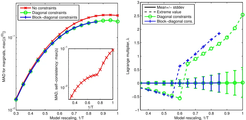
The alarm net is a pedagogical example of a graphical model that has been studied in the context of loop correction algorithms and is available in libDAI repository (see Mooij et al., 2007; Mooij, 2010). It has 37 variables, each variable takes either 2, 3 or 4 states (a mixture of Ising and Potts spins). Variables have biases, and participate in 2, 3 and 4 point interactions as shown in Figure 1 (upper graph). The model involves a mixture of factor types and variables. The Bethe approximation performs relatively poorly, due to short loops. We can again add a temperature and consider solutions up to the full scale
T = 1 that defines the model.
Two constraint regimes were applied: in the first pure-diagonal constraints were ap-plied: {(i, y),(i, y) : ∀i, y}, and in the second all block-diagonal constraints were applied {(i, y1),(i, y2) : ∀i, y1, y2}. The ability of both methods to improve local statistics were
0.2 0.3 0.4 0.5 0.6 0.7 0.8 0.9 1 −0.8
−0.6 −0.4 −0.2 0 0.2 0.4 0.6 0.8 1
Model rescaling, 1/T
Lagrange multiplier,
λ
Mean+/− stddev Extreme value Diagonal Off−diagonal Diagonal constraints On−and−off diag. cons.
0 0.2 0.4 0.6 0.8 1
10−4 10−3 10−2 10−1
MAD, self−consistency: max(
∆
)
Model rescaling, 1/T Diagonal, no constraints Off−diagonal error, no constraints Off−diagonal, diagonal constraints
Figure 8: A typical problem in the Wainwright Jordan set up forN = 16. (left) Negative
0.1 0.2 0.3 0.4 0.5 0.6 10−2
10−1
Model rescaling, 1/T
MAD for marginals, max(|
∆
(0
)|)
No constraints Diagonal constraints Median
Lower Quartile Upper Quartile
101 102
10−3
10−2
Number of variables,N
Root mean square Lagrange multiplier, \sqrt(E[\lambda^2])
T=5 T=5/2 T=5/3
Figure 9: Errors and Lagrange multipliers are shown for the states Potts model on 3-regular random graphs. (left) The diagonal constraint regime yields a significant improve-ment in maximum absolute deviation of p(xi) over the raw approximation on graphs with
0.3 0.4 0.5 0.6 0.7 0.8 0.9 1 10−2
10−1
MAD for marginals, max(|
∆
(0
)|)
Model rescaling, 1/T No constraints
Diagonal constraints Block−diagonal constraints
0.4 0.6 0.8 1
10−2 10−1
MAD, self−consistency: max(
∆
)
1/T
0.4 0.5 0.6 0.7 0.8 0.9 1
−1 −0.5 0 0.5 1 1.5 2 2.5 3
Model rescaling, 1/T
Lagrange multiplier,
λ
Mean+/− stddev Extreme value Diagonal constraints Block−diagonal cons.
Figure 10: Results for the alarm network. (left) The diagonal and block-diagonal constraint regimes have indistinguishable performance in the MAD for p(xi), and improve modestly on the unconstrained problem. (inset) At intermediate T there is a qualitative change in the self-consistency error, as some variable subsets become strongly polarized. (right) The values for λare for the most part small, with extreme values diverging asT approaches 1; a mixture of positive and negative Lagrange multipliers are required to enforce constraints.
5. Discussion
The aim of this paper is to show that for a range of models and variational methods we can have improved accuracy in marginal estimates by inclusion of a set of self-consistent constraints, and to propose this as a general mechanism by which to improve approximations with inconsistency between marginalization (first derivative) and linear response (second derivative) approximations.
We have expanded upon results for rather simple approximations, in easy to understand model frameworks: the marginals are improved in all cases, and in many scenarios by amounts measurable in orders of magnitude. The combination of a weak approximation method with constraints may result in there being no solutions and in marginal cases in a slow convergence of our proposed algorithm. On the other hand, if we are looking for a mechanism by which to leverage a good approximation this approach seems appropriate.
where the number of statistics available to constrain is large. Two directions are proposed in Appendix B.2.
Some powerful approximation methods are not variational and so the insight we provide cannot be leveraged. In other cases there is no inconsistency to exploit, this is true of adaptive-TAP and some moment matching methods. These have variational free energy frameworks, but by the Gaussian approximations therein used, there is a consistency of pairwise approximations, making redundant the constraints we suggest. This is in line with our thinking that good approximations should not violate these constraints.
We believe our method also sheds light on, or is inclusive of, previous attempts to leverage linear response. Consider the region-based free energy built on the set of regions indicated by Figure 2(d). Every outer region is a hub surrounded by leaves, and if we add constraints over the leaves within each region, a linear expansion in the Lagrange multipliers agrees with the linear expansion obtained in the scheme of Montanari and Rizzo (2005); however, outside of the linearized regime there are important differences.
There are three reasons one might not want to improve a variational approximation by adding self-consistency constraints: 1) The cost of the method which is dominated by a linear response evaluation (a cost that can be as large as O(N2) using susceptibility propagation), might be prohibitive in some applications. 2) Introducing such constraints may prevent the existence of any solutions (the method may reveal the uncomfortable truth that the approximation used is quite bad). 3) Even where a fixed point exists, it may be slow to reach it using a local iterative scheme forλsuch as (20).
6. Conclusion
We have demonstrated that adding covariance constraints, which make the linear response and marginalization estimates consistent, improves the performance of the Bethe approx-imation for a variety of simple model types. We have argued this is true more generally of variational frameworks, and have provided an algorithmic framework for mean-field and region-based frameworks, generalizing previous results. The regimes of adding all possible constraints (on-and-off diagonal) and adding constraints only over single variable covari-ances (diagonal) were examined. The former tends to lead to better results, whilst the latter is simpler to implement and can yield solutions across a broader range of models.
The usefulness of this paper is not in the specific algorithm developed, but in the princi-ple of statistical consistency. We hope it might be extended to other variational frameworks in which inconsistencies exist between first and second derivative estimates. We have pre-sented and tested an algorithmic framework; the framework can solve the constrained free energy where solutions exist, but a rather expensive (annealed in T) procedure was ex-ploited to obtain our results. Further work is required to make this reliable and competitive with state of the art marginal estimation.
Acknowledgments
Appendix A. Exact Expressions for the Fully Connected Ising model
It is straightforward to calculate the exact marginal distributions for (21), for any pair of variables
pT(xi, xj)∝ N−2
X
n=0
N −2
n
exp
(h+ [N−2−2n])2
2T +
1
Txixj+
h+ [N −2−2n]
T (xi+xj)
.
By contrast in the Bethe approximation
qij(xi, xj)∝exp
1
Txixj+ h→
T (xi+xj)
, (22)
where the log-ratio messagesh→ are defined as the solution to
h→=h+ (N −1)Tatanh [tanh(1/T) tanh(h→/T)] ; h→=
1 2log
µ
i→(ij)(1) µi→(ij)(−1)
.
Since we will place constraints on Vq(xi, xj) a convenient parameterization for the pair probability in our approximation will be
qij(xi, xj) =
(1 +Mixi)(1 +Mjxj) +Cijxixj
4 . (23)
We can restrict attention to symmetric solutions Mi = M and Cij = C, similarly at most two distinct Lagrange multiplier values need be considered: λi,i =λ0, when diagonal
constraints are applied, andλi,j =λ1 when off-diagonal constraints are applied. Minimizing
the variational free energy (17) with respect to M and C leads to the following pair of equations
0 = −[(n−1)M/T+λ0M] + atanh(M)+(N−1)
X
x1,x2
x1
2 qj(x2) log
qij(x1, x2) qi(x1)
,(24)
0 = −[1/T−λ1] +
X
x1,x2
x1x2
4 logqij(x1, x2). (25)
If we solve this pair of equations for λ = 0, we find an alternative representation of (22). Explicit expressions for the covariance matrix approximationχare derived in Raymond and Ricci-Tersenghi (2013b) and Raymond and Ricci-Tersenghi (2013a), these can be concisely expressed in the inverse as
[χ−1]i,j =
( 1
1−M2 h
1 + (n−1)(1−MC22)2−C2 i
−λ0 if i=j .
−1/T+P
x1,x2 x1x2
4 logqij(x1, x2)
− C
(1−M2)2−C2 otherwise.
Abbreviating χ−i,i1 = a and χi,j−1(j6=i) = b we can write the components of the covariance matrix approximation
χi,j =
1
(a−b)(a+ (N−1)b)
a+ (N−2)b if i=j .
Thus we have up to four parameters{M, C, λ0, λ1}, depending which constraints are applied.
We solve (24) and (25) in combination with either, or both, (1−M2 =χi,i) and (Cij =χi,j). These are non-linear equations inM,C and λ0; we resort to local search to find solutions;
solutions are possible by expansions at small or large T, or for largeN. For the solution to be valid, we also check that the Hessian is positive definite, and that p(xi, xj)≥0.
Solutions for the equations are trivial for large or smallT, and approach the solutions of the unconstrained approximation. By slowly varyingT we can discover the solutions that evolve continuously from these two fixed points. We did not find any solutions appearing discontinuously, nor did we find any evidence for symmetry breaking (that is solutions in which the magnetizations, or correlations, differed by label index).
It is also straightforward to apply the same methodology for the mean-field approx-imation: there is one saddle-point equation, (24) with C = 0; and up to one type of covariance constraint (χi,i= 1−M2), where the inverse covariance matrix elements become [χ−1]i,j =−1/T, and [χ−1]i,i= 1/(1−M2)−λ0.
Appendix B. Algorithm for Finding Optimized Lagrangian Parameters, and the Linear Responses
Our approach to find solutions depends on their existence, this is discussed generically before we consider the impact of constraint selection strategies (and constraint representation) on solution existence and algorithmic stablity. We then show that an exact method for minimizing the Lagrangian exists for some fixed values of the Lagrange parameters λ. The CLBP and CLSP algorithms are then presented in pseudocode. Finally, we discuss heuristics for the calculation of λ.
B.1 Existence
Certain models are known to be solved at leading order in some control parameter by region-based, Bethe or mean-field approximation. Examples are ferromagnetic random graphs or fully connected models in the limit of large number of variables (N), arbitrary models in the weakly interacting limit (also called high temperatureT), finite models in the limit of strong biases on the variables (h). In these models, we find, of course, that the deviation between the linear response and marginal estimates are small in the corresponding control parameter. Expanding in this parameter (for example 1/T, 1/N) it is straightforward to show the existence of solutions, and quantify the effectiveness of the constraints (see Raymond and Ricci-Tersenghi, 2013a). However, even outside the regime where expansions about the Bethe approximation are appropriate, we find solutions: this includes models where the covariance matrix has divergent terms, due to a mean-field phase transition as described in Raymond and Ricci-Tersenghi (2013b).
exist; applying all constraints is certainly a marginal case unless some are redundant. If we move to alphabets with more than 2 states per variable the number of pair-statistics for on-and-off diagonal constraints exceeds the number of variables (with no obvious redundancy); certainly such a system can have no solutions. We must think carefully on which constraints to implement, and this is discussed in Appendix B.2.
In the experiments of this paper we have introduced for all models the control parameter
T, with all models being well approximated by Bethe (and Mean-field) approximations in the weak coupling limit (T → ∞), and some models also being well approximated in the strong coupling limit (T → 0). To extend the regime in which our algorithms are convergent, an annealing approach was taken—slowly increasing 1/T (orT) and following a solution which evolved continuously in the marginals and Lagrange multipliers from the exactly solved regime. In many cases, solutions were found to reach a critical point T∗ beyond which they could not be continuously evolved to new solutions. At these points we invariably found no new solutions emerging discontinuously by simply iterating our procedures. By undertaking annealing, it would in principle be possible to miss some solution that emerges discontinuously; the example of Section 4.1 shows this is possible (there is coexistence of two solutions at low temperature for the case of off-diagonal constraints only), but in the other examples of this paper we found no evidence for this. We expect in most practical applications, and for good choices of the constraints, coexistence will be absent.
A common feature in solution discontinuity during annealing is the divergence of some Lagrange multiplier(s); this indicates that the failure was due to inviability of solutions rather than a breakdown of algorithmic dynamics. Unlike the Bethe approximation, which can be forced to converge to a local minimum at anyT, replacing LBP by a convex-concave procedure. We speculate that the constrained free energy has no solutions in strongly coupled regimes and that where practical solutions do exist the cavity based algorithms will be sufficient if combined with appropriate damping and/or annealing.
B.2 Selection of Constraints for Best Solutions
In this section we consider reasonable choices for the constraints, assuming a solution exis-tents, and algorithmic convergence is possible.
Since we are applying constraints to discrete models it is clear that the apriori constraints selection should be independent of the labeling convention. Furthermore, we note that we made the rather arbitrary choice in (2) of perturbations in the set of statistics {δxi,y :y= 1. . . Y},Y being the number of states. Whilst this is invariant under relabeling, and spans all possible perturbation directions (and one redundant direction P
yδxi,y), we might get different covariances according to our choice. It would seem sensible to choose our constraint regime so that any set of statistics that spans the set of perturbations yields the same result. To achieve this we must pick a complete basis{φ}, and apply constraints on all-covariance pairs.
The consideration of bases motivates the regimes we have explored: diagonal, off-diagonal, on-and-off diagonal. These schemes are basis-independent. If the condition
C(i,·),(j,·) = χ(i,·),(j,·) is met in one basis for all elements, then a change between two
We found that off-diagonal typically performed worse than on-diagonal, as well as being computationally more challenging. In the final experiment of Section 4.4 we also tried one basis dependent set of constraints, the so-calledpure-diagonalregime. Despite breaking the paradigm of basis independence, it performed just as well as theblock-diagonalregime that is basis independent, so this indicates that basis independence is not an essential feature in constraint selection.
Topological distinctions amongst constraints can also be made. In a region-based ap-proximation, we can distinguish the “2-core” from the rest of the graph. The 2-core is the set of variables that are found by recursively removing variables that are involved in at most one “outer region” (generalized interaction). We advise constraining variables on the 2-core only. The reason for this is that the set of variables that are not in the 2-core form a forest—a set of disconnected trees for which the approximation is conditionally exact even without constraints. If we have the core correct, then other constraints will be redundant. It is only in the case of the alarm net (Figure 1, Section 4.4) that the 2-core is distinguished from the full graph and we make this approximation. Other topological distinctions could be applied, distinguishing constraints by the distance between variables might be one pos-sibility (in Figure 2(b) for example there are nearest, and next nearest neighbors within the regions); however, in the Bethe approximation (all experiments we present) only nearest neighbors might be constrained so the example is mute.
Beyond these considerations, we did not attempt to further restrict the set of constraints in a model specific manner, but several options might be worth exploring, in particular: (1) Consider the covariance matrix restricted to a single variable “block”, χ(i,·),(i,·). For a
given approximation (for example Bethe) there is a unique orthonormal basis {φi} that diagonalizes the covariance matrix. This would provide a natural choice for the statistic basis. The eigenvalue-vector pairs determine which direction is most susceptible to a change in parameters, and so (loosely speaking) most sensitive to approximation errors. We might, therefore, rank constraints by this eigenvalues for inclusion. (2) If we can solve the problem to obtain qi∗, then we can consider defining only one perturbation statistic per variable as
φ(xi) ∝ log(Y q∗(xi)). Since we know approximations tend to be overconfident, it would seem a natural choice to constrain in line with the belief, rather than wasting resources on unimportant directions in parameter space.
B.3 Assignment of Constraints to Regions, and Basis selection, for Best Convergence
For our constraint regimes (diagonal, on-diagonal and on-and-off diagonal), the allocation of constraints to specific regions, the choice of statistical basis, the initial condition of the algorithm and the damping, leave the algorithmic fixed points unchanged. Owing to our slow annealing approach (increasing or decreasingT) our results were not very sensitive to the other implementation details. However, these choices do impact convergence significantly.