57
*Corresponding authoremail address: [email protected]
Assessment of different methods for fatigue life prediction of steel in
rotating bending and axial loading
J. Amiriana, H. Safarib, M. Shiranib,*, M. Moradia and S. Shabanib
aDepartment of Mechanical Engineering, Isfahan University of Technology, 84156-83111, Iran bSubsea Research and Development Center, Isfahan University of Technology, 84156-83111, Iran
Article info: Abstract
Generally, fatigue failure in an element happens at the notch on a surface where the stress level rises because of the stress concentration effect. The present paper investigates the effect of a notch on the fatigue life of the HSLA100 (high strength low alloy) steel which is widely applicable in the marine industry. Tensile test was conducted on specimens and mechanical properties were obtained. Rotating bending and axial fatigue tests were performed at room temperature on smooth and notched specimens and S-N curves were obtained. Using the obtained S-N curve for smooth specimens, the fatigue strength factor for the notched specimens were predicted by Weibull's weakest-link, Peterson, Neuber, stress gradient and critical distance methods and compared with experimental results. It was found that the critical distance and also Weibull’s weakest-link methods have the best agreement with experimental results.
Received: 24/01/2016 Accepted: 23/04/2016 Online: 03/03/2017
Keywords: Fatigue failure, S-N curve, Rotating bending.
1. Introduction
A component with an unchanging cross-sectional area under a load has a uniform and homogeneous stress and strain distribution. Any type of notch existence or sudden changes in cross-section causes an inhomogeneous distribution of stress and strain. In general, fatigue failure in an element arises where the stress level rises due to the stress concentration effect such as a notch on a surface. Notch is usually defined as a geometric discontinuity. A notch may be introduced either by designing or by a manufacturing process. A hole in a component is an example of a designed notch.
Fabrication defects such as weld defects, inclusions, casting defects, or machining marks are notches which are introduced due to the manufacturing process [1].
58
[3] and critical distance method presented by Taylor [4] are two other methods proposed for. Critical distance method is based on the critical distance at the notch root. These methods are mainly based on empirical tests, which are conducted on many metals.
It should be considered that these methods are not consistent with finite element results. This shortcoming is solved by weakest-link theory presented by Weibull, in which the probability of fatigue failure is obtained from finite element results [5-10]. In Weibull's weakest-link theory, critical defects are assumed statistically scattered in the volume of a component. In this theory, the size of defects is supposed very small compared to the distance between them and therefore the defects do not interact [11-13]. Just as a chain is as strong as its weakest link, the fracture of the weakest link yields the failure of a complete component. Therefore, the weakest-link theory supposes that probability of survival of the whole component equals to the production of the probabilities of survival of all the elements. In this study, HSLA100 (high strength low alloy) steel is investigated. This material is applicable in marine industry, where different types of severe fatigue loading are applied on the marine structure during its life; therefore, accurate life investigation of this steel is essential for the marine industries [14, 15].
HSLA steels are designed to deliver particular advantageous mixtures of properties such as toughness, strength, weldability, formability and atmospheric corrosion resistance. In order to retain formability and weldability, carbon content in HSLA steel is between 0.05–0.25 percent [16, 17]. HSLA100 steel is designed for the yield strength ≥
700MPa and impact strength ≥/ 81 J at 84 °C [18,
19].
The main goal of this research is to compare different methods of predicting fatigue life of notched HSLA100 specimens and find which ones yield better results. In order to do that, fatigue tests were conducted on smooth and notched specimens
to obtain the S-N curves. Neuber, Peterson, stress
gradient, critical distance and Weibull's weakest-link methods were used to predict the S-N curve
for the notched specimens based on the S-N curve
for smooth specimens. The obtained theoretical results were compared with experimental data.
2. Experimental procedure
2.1 Material Properties and specimens
Experimental results obtained from testing were used for analysing and comparing with the
theoretical methods. Tensile tests were
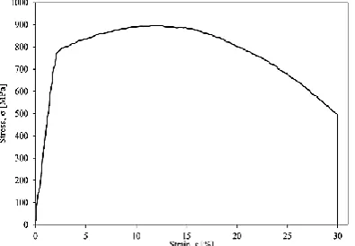
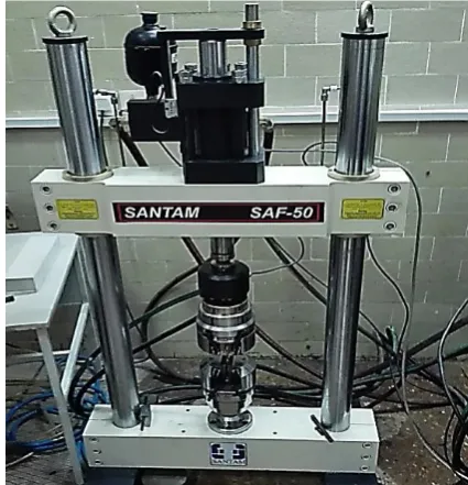
performed according to ASTM E8 [20] and mechanical properties of the studied material were obtained. Figure 1 shows a typical engineering stress-strain curve for the tested steel and Fig. 2 shows the test equipment. Tables 1 and 2 summarize the mechanical properties and chemical composition of the used material, respectively.
Rotating bending [21] and axial fatigue tests [22] were carried out on smooth and notched specimens. Figure 3 shows dimensions of the smooth and notched cylindrical specimens for rotating bending and axial fatigue tests.
Fig. 1. The engineering stress-strain curve for the tested steel.
59
Table 1. Mechanical properties of the studied HSLA100.
Yield strength Sy (MPa)
Ultimate strength Su (MPa)
Strain at break Eu (%)
Modulus of elasticity E (GPa)
791 895 31 197
Table 2. Chemical composition of the studied HSLA100 (wt %.).
Ni Mn Cu Cr Mo Si C Nb Al
3.59 0.91 1.59 0.59 0.58 0.25 0.03 0.03 0.02
Fig. 3. Detailed drawings of specimens; (a) smooth and (b) notched specimens (all dimensions are in mm).
2.2 Fatigue tests
In the rotating bending test, a constant load was applied perpendicular to the cylindrical specimen rotating at 50 Hz. In the axial test, the cylindrical specimen was cyclically loaded to the failure by servo-hydraulic testing machine using a sinusoidal signal. Fourteen smooth and twelve notched specimens were rotating bending and axially fatigue tested each. Experimental equipment used for testing smooth and notched specimens are shown in Fig. 4 and 5.
2.3 Test results
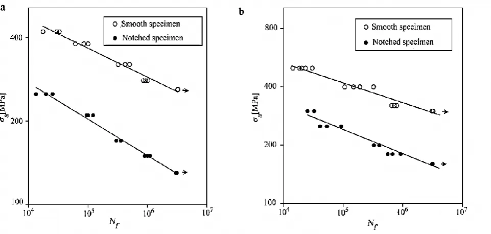
Fatigue test results are presented in Fig. 6. The number of cycles before failure, Nf, was plotted against the net section stress amplitude, σa. Based on the rotating bending test data, fatigue limit for the smooth and notched cylindrical specimens are
310MPa and 170MPa, respectively. Also, based on the axial test data, fatigue limit for the cylindrical smooth and notched specimens are 270MPa and 140MPa respectively. Fatigue strength factor (kf) for the notched specimen in rotating bending and axial fatigue tests are 1.82 and 1.93, respectively. kf is obtained by dividing fatigue limit of smooth specimen to fatigue limit of notched specimen. The fatigue strength factor (kf) is a function of the notch geometry and the type of loading.
Fig. 4. Experimental equipment for rotating bending tests
Fig. 5. Experimental equipment for axial tests
60
(1) log(σa)=-0.1073log(Nf) + 3.1588
and for the notched specimen is:
(2) log(σa)=-0.1295 log(Nf) + 3.0239
Also, line equation passing through the axial fatigue test results for the smooth specimens, is as follow:
(3) log(σa)=-0.1041 log(Nf)+3.0843
and for notched specimen is:
(4) log(σa)=-0.131 log(Nf) + 2.9626
Usually, Basquin equation is used to describe the
S-N curve in the high-cycle-region. Basquin
equation is as follow:
(5)
σa=σf′(Nf)
−1
m
where σf'is the fatigue strength coefficient and
-1 /m is the fatigue strength exponent. This curve
will be a straight line on a log-log plot and may be found by linear regression analysis of fatigue data points. The logarithm of Eq. (5), gives the following linear relationship:
(6) log(σa)= log(σf')-1
mlog(Nf)
or
(7)
y(x)=ax+b
with
y(x)=log(σa), x= log(Nf), a=-m1,b= log(σf'). By comparison of line equations for smooth and notched specimens with Eq. (6), the fatigue strength coefficient and the fatigue strength exponent in rotating bending fatigue will be
m=9.34, σf'=1441.45 for the smooth specimens,
and m=7.75, σf'=1056.8 for the notched specimens. Also, the fatigue strength coefficient and the fatigue strength exponent in axial fatigue will be
m=9.61, σf'=1214.2 for the smooth specimens, and
m=7.63, σf'=917.5 for the notched specimens.
Fig. 6. Fatigue behaviour of the HSLA100 cylindrical specimens with and without notch (a: rotating bending loading and b: axial loading).
61
3. Prediction of notch effect on fatigue life of HSLA100 specimens
In this section, Weibull's weakest-link, Neuber, Peterson, stress gradient and critical distance methods are used to predict notch effect on fatigue life of the HSLA100 steel. Stress concentration factor, kt, is required to use Neuber, Peterson and stress gradient methods. This factor is obtained by simulation of stress distribution for both smooth and notched specimens by finite element method.
kt is obtained by dividing maximum stress at the
notch root by average cross section stress.
Stress concentration factor for the notched
specimen, Fig. 3, is kt =2.73 for the bending load
and kt =2.86 for the axial load. However, the tests indicated that at the fatigue limit, the presence of a notch on a component under cycling nominal stresses reduces the fatigue strength of the smooth component by a factor of kf and not the factor of kt. A formula, which is acceptable in engineering applications and expresses fatigue strength factor is as follow [1]:
(8)
kf=1+q(kt-1)
As can be seen, this formula empirically relates fatigue strength factor to the elastic stress concentration factor by a notch sensitivity factor q. In critical distance method, it is required to determine stress gradient at the notch root. So the bending and axial load were applied on the notched specimen and stress gradient was obtained.
3.1 Weibull’s weakest-link theory
In the weakest link theory, the probability of component failure [5] is described as:
(9)
pf,v=1-exp[-( σ̅a σ*A
0 )
bσ ]
Equation (9) is called Weibull fatigue strength distribution and corresponds to a two-parameter Weibull distribution. bσ, is the Weibull shape or shape parameter and refers to the measure of reference specimens fatigue strength scatter. σ*A0,
is the scale parameter and refers to the fatigue characteristic of the reference fatigue test
specimen. σa is the Weibull stress amplitude and
illustrate the fatigue-effective stress amplitude. There are two different methods based on the weakest link theory for estimating the probability of failure of specimens [5, 23]. In the first approach, called the volume method, the critical defect is assumed to lie somewhere within the volume of the specimen. In the second approach, the controlling defects are assumed to be located on the surface of the specimen. This approach is therefore called the surface method.
In the volume formulation of Weibull's weakest-link method, σais defined as:
(10)
σ̅a=(v1 0∫σa
bσ
v 𝑑𝑣)
1 bσ
where v0 is an arbitrary reference volume or the
volume of reference fatigue test specimen and v is
the component volume.
In the surface formulation of Weibull's weakest-link method, σais defined as:
(11)
σ̅a=(𝐴1 0
∫σabσ𝑑𝐴
A )
1 bσ
where A0 is an arbitrary reference surface or the surface of reference fatigue test specimen and 𝐴 is the component surface. Weibull fatigue strength distribution (Eq. (9)) can be transformed into a Weibull fatigue life distribution through the Basquin equation (Eq. (5)), and finally Weibull fatigue life distribution will be obtained as follow:
(12)
Pf,v=1-exp[-(N* n 0(R,σ̅ )a )
bn ]
where bn and N*0 are shape parameter and scale parameter, respectively. The bn is related to bσby following equation:
(13)
62
where m is the fatigue strength exponent.
Weakest-link theory assumes that if the component is divided into small elements, the probability of survival of a component is the product of the probabilities of survival of the (small) elements. The probability of survival of an element is a function of the stress cycle, the fatigue strength characteristic, material scatters and also the size of the element.
For applying the weakest-link theory, an in-house developed software was used in this research. This software is a fatigue post-processor which uses the results from a standard finite element stress analysis. In order to compute the fatigue life of a component by this software, the required inputs are as follows:
Mechanical properties of the HSLA100
(ultimate strength, fatigue strength) obtained from the tensile and fatigue tests in section 2.
The parameters of S-N curve for the smooth
specimen (fatigue strength coefficient, fatigue strength exponent) obtained from the rotating bending and axial fatigue tests in section 2.
Weibull constants for the smooth specimen
(-shape parameter, scale parameter) which will be obtained in section 3.1.
Finite element file of the simulated notched specimen (a file containing the element topology, nodal coordinates, and nodal coordinate stresses) which will be explained in section 3.2.
The volume of reference fatigue test specimen v0
and the surface of reference fatigue test specimen
𝐴0, in this research, is calculated as 1536 mm3 and
1053 mm2, respectively.
3.1.1. Statistical analysis of fatigue data to find the Weibull distribution constants
In this section, statistical analysis of fatigue test results is performed to find the Weibull distribution constants. If several specimens are tested until fatigue failure, the obtained fatigue lives will differ from specimen to specimen. If a sufficient number of test specimens at each stress level are available, and then the Weibull distribution is fitted to each stress level, an S-N curve for different probabilities of failure can be obtained [24]. In this research, 14 smooth specimens were tested in two rotating bending and axial fatigue tests each. This number of
replications was not sufficient to create S–N curves for different probabilities of failure at each stress level. Therefore, a special curve fitting technique used by the authors in their other published works
was applied [25]. S–N curves for various
probabilities of fatigue failure will be moved by a uniform value in the vertical direction (stress direction) if it is supposed that the coefficient of variation in strength is constant. Thus, as shown in Fig. 7, if k data points are accessible, it is practical
to move k parallel S–N curves (on a log-log plot)
through these data points and from each S–N curve
one probability of failure will be obtained.
With this technique, different probabilities of fatigue failure (k) can be obtained and at each fatigue strength, σa, there will be k number of life values. Then by applying Weibull distribution to these k lives at an arbitrary stress level, bn and N*0
are obtained for the studied material (bn=2.78,
N*
0=5.76×10⁵ for the rotating bending load and
bn=2.71, N*0=5.96×10⁵ for the axial load). Also with these two values (bn and N*0) and using Eq. (5 and 13), bσ and σ*A0 are obtained (bσ=25.91,
σ*
A0=347.32 for the rotating bending load and
bσ=26.04, σ*A0=304.55 for the axial load). It should be noted that m and σf'belong to the smooth specimen equation. In the following sections, it will be explained how parallel S-N curves are drawn.
63
(14)log(Nf)= -8.90log(σa)+28.35
and for axial load is:
(15) log(Nf)= -9.36 log(σa)+29
The slope of these parallel S-N curves is equal to the slope of the rotating bending S-N curve and the axial S-N curve, -8.90 and -9.36 respectively.
3.1.2 Stress analysis of axial and rotating bending notched specimen
In axial fatigue loading, stresses can easily be obtained. In the weakest link theory, maximum stress in notched specimen under fatigue loading is required. This can be obtained by the use of available commercial finite element softwares. Therefore, the notched specimen is simulated in the finite element software under axial loading and the stresses are calculated.
But stress amplitude distribution in an
axisymmetric specimen under rotating bending cannot directly be obtained by a finite element analysis.
However, by superimposing suitably weighted FEA stress distributions from bending about the
y- and z-axes, Fig. 7, the stress amplitude
distribution in rotating bending can be readily obtained [27].
A bending moment M is applied to a rotating cylindrical specimen. Cross section of this specimen is shown in Fig. 8. At the particular instant, the radius OA is perpendicular to the moment vector and the axial stress at this moment (point A in Fig. 8) reaches its maximum. During rotating bending, the stress state at the position x for an arbitrary angle of rotation (point
A), θ, is:
(16 )
σx(A)=M
cosθ . OAcosθ
I +
Msinθ . OAsinθ I
or
(17)
σx(A)=σMy(A)cosθ+σMz(A)sinθ
where σMy(A) and σMz(A) are the resulting stress
tensor fields for bending around the specimen's y-
and z-axis, respectively for point A. y and z are perpendicular to each other and also to the length axis (x-axis) of the specimen.
64
The stress fields σMy(A) and σMz(A) can be determined by means of two separate load cases for a finite-element model of the rotating bend specimen. Similarly, for all points of the specimen (all nodes of the simulated specimen by finite element method) the stress field is obtained. By applying the above-mentioned methodology, an axisymmetric stress field is obtained for the notched specimens, Fig. 9, to be used in the weakest-link analysis.
Fig. 8. Cross-section of a rotating bending specimen subjected to a bending moment M.
Fig. 9. Stress distribution for the notched specimen; (a) rotating bending load and (b) static load.
3.1.3 Weibull's weakest-link results
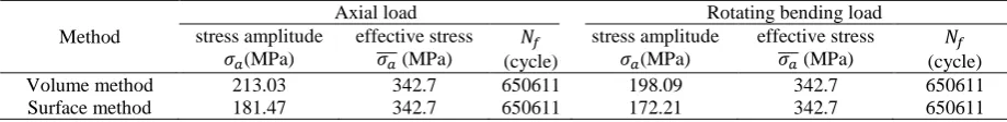
kf in weakest-link theory is obtained by dividing the effective stress to the stress amplitude. As specified in Table 3, the surface method yields
more conservative predictions than the volume method. The fatigue-effective stress amplitude is calculated by integrating the stress over the surface in the surface method and over the volume for the volume method. Since surface stresses are larger than volume stresses, the calculated fatigue-effective stress amplitude in the surface method is larger than volume method at the same applied stress amplitude.
3.2 Peterson method
Peterson assumes that fatigue failure occurs when stress at a point in a critical distance (ap) away from the notch root is equal to the fatigue strength of a smooth specimen. The following empirical equation is proposed for q:
(18)
q= 1
1 +arp
where ap is the material constant which is
dependent on the loading and size and r is the
notch root radius [28]. ap is obtained from
experimental curves that are provided by Peterson [28]. By applying Eq. (8 and 18), the fatigue strength factor for the rotating bending and axial fatigue tests is obtained 2.09 and 2.17, respectively.
3.3 Neuber method
In Neuber method [29] it is assumed that fatigue damage occurs if the average stress over a distance (an) from the notch root equals to the fatigue limit of a smooth specimen. Neuber presented the
following empirical equation for q:
(19)
q= 1
1 +√arn
where r is the notch root radius and an is the
65
Table 3.Weibull's weakest-link results for probability of fatigue failure of 50 percent.
Method
Axial load Rotating bending load stress amplitude
𝜎𝑎(MPa)
effective stress 𝜎𝑎
̅̅̅ (MPa)
𝑁𝑓 (cycle)
stress amplitude 𝜎𝑎(MPa)
effective stress 𝜎𝑎
̅̅̅ (MPa)
𝑁𝑓 (cycle) Volume method 213.03 342.7 650611 198.09 342.7 650611 Surface method 181.47 342.7 650611 172.21 342.7 650611
3.4 Stress gradient method
Siebel and Stieler [3] used the stress gradient effects on the fatigue strength reduction instead of the notch root radius. They introduced a new parameter, the relative stress gradient (RSG), defined as follow:
(20)
RSG= 1
σe(x)(
dσe(x)
dx )x=0
where x is the normal distance from the notch root
and σe(x) is the theoretically calculated elastic stress distribution. By testing fatigue strength of the smooth and notched specimens, they provided
empirical curves relating k kt / f to RSG for
various materials. These curves can be expressed by the empirical formula. The fatigue strength factor for the rotating bending and axial fatigue tests is obtained 2.53 and 2.66, respectively.
3.5 Critical distance method
Theory of critical distance contains three different approaches [4]. This section starts with point method and then the line method and area method. In these methods, the stress gradient in front of the notch root and a critical distance from the notch root are required. Stress gradient in front of the notch root obtained by finite element analysis and critical distance is as follow:
(21)
L=1π(∆kth
∆σ0)
2
This equation relates critical distance to two materials constants, Δkth and Δσ0, where Δkth is stress intensity threshold and Δσ0 is fatigue limit.
Distance on the stress–distance curve is denoted by
r and stress by Δσ(r).
According to the point method, fatigue failure occurs when the stress value reaches the strength of a smooth specimen in half of the critical distance, i.e.:
(22)
∆σ(r=𝐿
2)=∆σ0
In the line method, the average stress over r = [0,𝐿 2⁄ ] is used, and fatigue failure occurs when this average stress is equal to the strength of a smooth specimen. The area method involves averaging the stresses over some areas in the vicinity of the notch. In the area method, fatigue failure occurs when this average stress is equal to the strength of a smooth specimen [4].
To obtain critical distance, the stress intensity threshold (Δkth) and the fatigue limit (Δσ0) should be available, but the stress intensity threshold of HSLA100 is not available; therefore, an alternative method is used.
Peterson [28] presented an empirical equation that relates critical distance to ultimate strength for bending load:
(23)
𝐿(𝑚𝑚) = 2 × 0.0254 ×( 2079
su (MPa)) 1.8
Through this method, for the HSLA100, the critical distance is obtained (L=0.2316). Since in critical distance method it is required to calculate
stress gradient at the notch root,
66
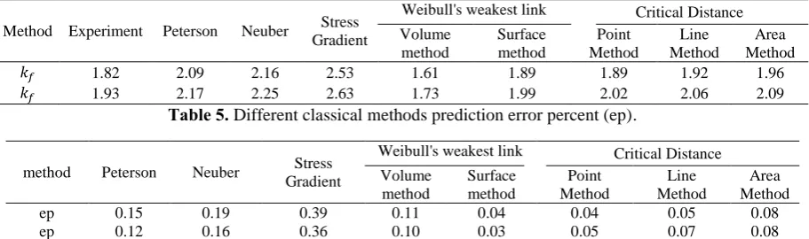
Table 4. Fatigue strength factors (kf) predicted by experiments and also different methods.
Method Experiment Peterson Neuber Stress Gradient
Weibull's weakest link Critical Distance
Volume method
Surface method
Point Method
Line Method
Area Method 𝑘𝑓 1.82 2.09 2.16 2.53 1.61 1.89 1.89 1.92 1.96 𝑘𝑓 1.93 2.17 2.25 2.63 1.73 1.99 2.02 2.06 2.09
Table 5. Different classical methods prediction error percent (ep).
method Peterson Neuber Stress Gradient
Weibull's weakest link Critical Distance
Volume method
Surface method
Point Method
Line Method
Area Method ep 0.15 0.19 0.39 0.11 0.04 0.04 0.05 0.08 ep 0.12 0.16 0.36 0.10 0.03 0.05 0.07 0.08
stress gradient at the notch root,
the bending and axial load are applied on the notched specimen.
The obtained fatigue strength factor, kf, in rotating bending fatigue is 1.89, 1.92, and 1.96 for point, line, and area methods, respectively. In axial fatigue, this factor is 2.02, 2.06, and 2.07 for point, line, and area methods, respectively.
4. Results and discussion
The predicted fatigue strength factors of the foregoing analysis are summarized in Table 4. Also different classical methods prediction error percent have been summarized in Table 5. According to Tables 4 and 5, the fatigue strength factors predicted by critical distance and Weibull's weakest-link methods are the closest to the experimental results. But it should be noted that to apply critical distance, stress intensity threshold is required which is not available for the studied material. Therefore, an empirical equation is used to obtain critical distance. Neuber, Peterson, and stress gradient methods are the mainly empirical approaches and easy to use. According to Tables 4 and 5, the predictions made by these methods are conservative, which is some consolation for engineering designers, but nevertheless, the errors are high.
It should be considered that these methods are not consistent with the finite element results. To select an appropriate method of assessing the notch effect in components subjected to fatigue, availability of the required materials data, the predictive
capability and the compatibility with FEA stresses are usually the most important criterion for a design engineer. So with considering these points, Weibull’s weakest-link theory is recommended to predict fatigue life among the studied methods in this research.
5. Conclusions
Tensile, axial and rotating bending fatigue tests were conducted on cylindrical specimens. Fatigue experiments were carried out on two sets of -notched and smooth specimens in rotating bending and axial fatigue loads. The material under investigation was HSLA100 steel, which is widely applicable in the marine industry. Mechanical properties of the HSLA100 steel and fatigue properties for notched and smooth specimens were presented. Notch effect on fatigue strength of the HSLA100 steel in rotating bending and axial
fatigue loads was experimentally evaluated, and S–
N curve was obtained.
Weibull's weakest-link, Neuber, Peterson, stress gradient and critical distance methods were used to predict fatigue strength factor for the notched specimen based on the obtained S-N curve of the smooth specimen. The obtained theoretical results were compared with experimental data. It was found that the critical distance and Weibull’s weakest-link methods have the best agreement with experimental results.
References
[1] Y. L. Lee, J. Pan, R. Hathaway and M.
67
theory and practice, 1st ed., Elsevier, Oxford, (2005).
[2] N. E. Dowling, Mechanical behavior of
materials - engineering methods for deformation, fracture, and fatigue, 3rd ed., Prentice Hall, New Jersey, (2007).
[3] E. Siebel and M. Stieler, “Ungleichförmige
Spannun gsverteilungbeischwingender
Beanspruchun-g”, VDI-Z . Vol. 97, No. 5, pp.121-126, (1955).
[4] D. Taylor, The theory of critical distances -
a new perspective in fracture mechanics,1st ed., Elsevier, London, (2007).
[5] A. Wormsen, B. Sjödin, G. Härkegård and
A. F. jeldstad,“Non-local stress approach for fatigue assessment based on
weakest-link theory and statistics of
extremes”,Fatigue Eng. Mater. Struct, Vol.
30, No. 12, pp.1214-1227, (2007).
[6] W. Weibull, “A statistical theory of the
strength of materials”, IVA Handlingar,Vol.
151, pp.1-45, (1939).
[7] W. Weibull,“The phenomenon of rupture in
solids”, IVA Handlingar,Vol. 153,
pp.155-160, (1939).
[8] W. Weibull,“A statistical distribution
function of wide applicability”,Appl. Mech.
Eng, Vol. 18, No. 3, pp.293-297, (1951).
[9] M. Shirani and G. Härkegård,“Large scale
axial fatigue testing of ductile cast iron for heavy section wind turbine components”,
Eng. Failure Anal,Vol. 18, No. 6, pp.1496-1510, (2011).
[10] M. Shirani and G. Härkegård,“Fatigue life distribution and size effect in ductile cast
iron for wind turbine components”,Eng.
Failure Anal, Vol. 18, No. 1, pp.12-24, (2011).
[11] M. Shirani and G. Härkegård,“Damage tolerant design of cast components based on defects detected by 3D X-ray computed
tomography”,Int. J. Fatigue, Vol. 41,
pp.188-198, (2012).
[12] M. Shirani and G. Härkegård, “Casting defects and fatigue behaviour of ductile cast iron for wind turbine components: A
comprehensive study”, Materialwiss.
Werkstofftech,Vol. 42, No. 12, pp.1059-1074, (2011).
[13] M. Shirani and G. Härkegård, “Fatigue crack growth simulation in components
with random defects”, J. ASTM In, Vol. 6,
No. 9, pp.1089-1121, (2009).
[14] T. Montemarano, B. Sach, J. Gudas, M.
Vassilaros and H. Vandervelt, J. Ship Prod,
Vol. 2, No. 3, pp.145, (1986).
[15] HSLA Steel, 2002-11-15, archived from the original on 2010-01-03, retrieved 2008-10-11.
[16] J. Davis, Alloying: Understanding the
Basics. ASM International, (2001).
[17] S. Mikalac and M. Vassilaros, Proc. Of Int. Conf. on Processing, Microstructure and Properties of Microalloyed and Other Modern High Strength Low Alloy Steels, Iron and Steel Society, Pittsburgh, PA, June 3-6. p. 331 (1991).
[18] A. Coldren and T. Cox, “Technical Report”,
David Taylor Research Laboratory,
DTNSRDCN00167-85-C-006, (1985). [19] E. Czyryca, Proc. Conf. on Advances in
Low Carbon High Strength Ferrous Steels LCFA-92, O.N. Mohanty, B.B. Rath, M.A. Imam, C.S. Sivaramakrishnan (Eds.), Indo-US Pacific Rim Workshop, Trans Tech Pub., Jamshedpur, India, March 25-28, p. 490, (1992).
[20] ASTM Standard E8. Standard Test Methods for Tension Testing of Metallic Materials. West Conshohocken (PA, USA): ASTM International, (2007).
[21] ASTM Standard E2948-14. Standard Test Method for Conducting Rotating Bending Fatigue Tests of Solid Round Fine Wire. West Conshohocken (PA, USA): ASTM International, (2007).
[22] ASTM Standard E 466-07. Standard practice for conducting force controlled constant amplitude axial fatigue tests of metallic materials. West Conshohocken (PA, USA): ASTM International, (2007).
[23] H. Belmonte, M. Mulheron, P.
Smith,“Weibull analysis, extrapolations and implications for condition assessment of
cast iron water mains”,Fatigue Eng. Mater.
Struct. Vol. 30, No. 10, pp. 964-90, (2007).
[24] W. Weibull,Fatigue testing and analysis of
68
[25] S. Nishijima,“Statistical fatigue properties of some heat-treated steels for machine structural use”,ASTM Spec Technol Publ. Vol. 744, pp.75-88, (1981).
[26] J. Wilson,“Statistical comparison of fatigue data”, J. Mater. Sci. Lett, Vol. 7, No. 3, pp. 307-308, (1988).
[27] G. Härkegård and G. Halleraker, “Assessment of methods for prediction of notch and size effects at the fatigue limit
based on test data by Böhm and Magin”,Int. J. Fatigue.Vol. 32, No. 10, pp.1701-1709, (2010).
[28] R. E. Peterson,Notch sensitivity. In: Sines G, Waisman JL, editors. Metal fatigue. McGraw Hill, New York, (1959).
[29] H. Neuber,Theory of notch stresses - principles for exact calculation of strength with reference to structural form and material, Springer, Berlin, (1958).
How to cite this paper:
J. Amirian, H. Safari, M. Shirani, M. Moradi and S. Shabani,“Assessment of different methods for fatigue life prediction of steel in rotating bending and axial loading ”, Journal of Computational and Applied Research in Mechanical Engineering, Vol. 6. No. 2, pp. 57-68
DOI: 10.22061/jcarme.2017.597