Application of Conditional Autoregressive Value at Risk Model to Kenyan Stocks: A Comparative Study

(1)

http://www.sciencepublishinggroup.com/j/ajtas doi: 10.11648/j.ajtas.20170603.13

ISSN: 2326-8999 (Print); ISSN: 2326-9006 (Online)

Application of Conditional Autoregressive Value at Risk

Model to Kenyan Stocks: A Comparative Study

Winnie Mbusiro Chacha, P. Mwita, B. Muema

Department of Statistics and Actuarial Science, Jomo Kenyatta University of Agriculture and Technology, Nairobi, Kenya

Email address:

[email protected] (W. M. Chacha)

To cite this article:

Winnie Mbusiro Chacha, P. Mwita, B. Muema. Application of Conditional Autoregressive Value at Risk Model to Kenyan Stocks: A Comparative Study. American Journal of Theoretical and Applied Statistics. Vol. 6, No. 3, 2017, pp. 150-155.

doi: 10.11648/j.ajtas.20170603.13

Received: October 28, 2015; Accepted: November 6, 2015; Published: May 22, 2017

Abstract:

Value at Risk (VaR) became the industry accepted measure for risk by financial institutions and their regulators after the Basel I Accords agreement of 1996. As a result, many methodologies of estimating VaR models used to carry out risk management in finance have been developed. Engle and Manganelli (2004) developed the Conditional Autoregressive Value at Risk (CAViaR) which is a quantile that focuses on estimating and measuring the lower tail risk. The CAViaR quantile measures the quantile directly in an autoregressive framework and applies the quantile regression method to estimate the CAViaR parameters. This research applied the asymmetric CAViaR, symmetric CAViaR and Indirect GARCH (1, 1) specifications to KQ, EABL and KCB stock returns and performed a set of in sample and out of sample tests to determine the relative efficacy of the three different CAViaR specifications. It was found that the asymmetric CAViaR slope specification works well for the Kenyan stock market and is best suited to estimating VaR. Further, more research needs to be carried out to develop e a satisfactory VaR estimation model.

Keywords:

VaR, Asymmetric CAViaR, Symmetric CAViaR, Indirect GARCH (1, 1) CAViaR

1. Introduction

Global financial markets and financial institutions have lately been faced with the turmoil of extreme and unexpected movements in security’s prices which has resulted in loss of wealth to investors, bankruptcy, market crashes and even economic crises. This is evidenced by the 1720 south sea bubble, the stock market crash on Wall Street in October 1987, the 1997 Asian financial crisis, and from the recent global economic crisis of 2007-2008.

These unexpected price movements causing extreme risk though rare, are of great importance in modern risk management and decision making in financial institutions and to their regulators. Hence, understanding of the expected frequency and magnitude of the financial extremes causing the downside risk is crucial.

Financial institutions are exposed to several types of risk such as market risk, liquidity risk, operational risk and credit risk. The exposure to market risk, which is the risk exposure brought about by changes in asset prices or liabilities, was of focus in this work. The study focuses on market risk because

an accurate estimation of market risk will enable financial institutions to maintain capital requirements that meet the underlying market riskexposure that they face.

VaR was first introduced by J.P Morgan in Risk Metrics in 1996 then later on adopted in the Basel I Accords. VaR has two main objectives, namely, to measure the market risk and to determine the minimum capital reserve. VaR is used for portfolio management, auditing and risk hedging. To provide a comprehensive assessment of risk, several VaR measures can be computed, for a set of different risk levels such as = 1%; 5%, etc., and over a set of different horizons, such as h = 1, 10, 20 days, (Gourieroux & Jasiak, 2010).

(2)

of investment opportunities available at the NSE it is essential to have a robust estimation method of VaR to minimize losses that could face the investors.

Moreover, previously existing methods of VaR estimation such as the Risk Metrics model which is a standard tool to measure market risk within financial institutions have weaknesses that could result in the under estimation or over estimation of VaR, (Abad et al., 2014). Further, Thupayagale (2010) observes that different VaR methodologies work well for different countries.

The study seeks to identify which of three CAViaR specifications introduced by Engle & Manganelli (2004), that is, the asymmetric CAViaR specification, the symmetric CAViaR specification and the indirect GARCH (1,1) work well in the Kenyan stock market. We applied the CAViaR models to estimate the VaR. The CAViaR incorporates the autoregressive property of VaR as a result of the autocorrelation of the distribution of returns due to volatility clustering in the returns. The parameters of the CAViaR quantile are estimated using regression quantiles introduced by (Koenker & Bassett, 1978). In the auto-regression case, the use of the CAViaR quantile which models the VaR quantile directly helps to overcome the issue of the quantile regression not applying sufficiently far in the tails (Allen et al., 2012).

The research assesses which CAViaR model accurately estimates the VaR using three stocks namely KQ, KCB and EABL. In so doing, the percentage of times VaR is exceeded at the 99 % and 95% high probability level over a one day time horizon was established.

2. Literature Review

Engle & Manganelli (2004) developed a parametric approach to VaR estimation whereby the estimation of VaR uses the notion of conditional autoregressive specification of the VaR which they refer to as Conditional Autoregressive Value at Risk (CAViaR). In the CAViaR, instead of modelling the whole distribution, they model the quantile directly in an autoregressive framework. Since financial returns exhibit volatility clustering, this statistically implies that the returns are also auto-correlated hence VaR which is linked to the standard deviation of the returns also is auto-correlated thus the use of the autoregressive specification.

Huang et al. (2009) apply CAViaR to forecasting oil price risk. In doing so, they provide two original contributions by introducing a new exponentially weighted moving average CAViaR model and developing a mixed data regression model for multi-period VaR prediction.

Allen et al. (2012) apply the CAViaR model to Australian stocks and contrast the results with those of a GARCH (1, 1) model, the Risk Metrics model and the APARCH model. They find that the CAViaR model works well for his dataset apart from periods of the global financial crisis. He further finds that the behavior of the tail is different from the rest of the distribution.

Chen et al. (2012) propose novel nonlinear threshold

conditional autoregressive VaR (CAViaR) models that incorporate intra-day price ranges. Model estimation is performed using a Bayesian approach via the link with the skewed Laplace distribution. The performances of a range of risk models during the 2008-09 financial crisis were examined, including an evaluation of the way in which the crisis affected the performance of VaR forecasting. The proposed threshold CAViaR model, incorporating range information, is shown to forecast VaR more effectively and more accurately than other models, across the series considered.

White et al. (2010) study a multivariate extension of CAViaR, which lends itself to estimating dynamic versions of CoVaR.

On the contrary, CAViaR models cannot be used for volatility forecasts which is important in applications such as option pricing. In the context of forecast evaluation, Taylor (2005) furthers the CAViaR model to construct the financial volatility forecasts using the approach of approximating the conditional volatility by a simple time-invariant function of the interval between CAViaR forecasts of symmetric quantiles.

Koenker & Bassett (1978) developed the regression quantiles. The regression quantile is basically a simple minimization problem yielding the sample quantile. The solution to the minimization problem are the estimators of the parameters. They suggest estimators of the regression quantile that have an efficiency that is comparable to and proved to outperform the efficiency of the least squares Gaussian model estimators. The regression quantile approach is used to estimate the parameters of the CAViaR model in this research.

3. Methodology

The return of portfolio with price process yt over the time period [t; t - 1] is given by:

= ln ( ).

The research focuses on three of the CAViaR model specifications applied to Kenyan stock to test the relative suitability of the three models in calculation of VaR

3.1. Asymmetric Slope (AS)

= ( )

= + + ( ) + ( )

Where ( ) and ( ) are positive and negative returns respectively.

(3)

3.2. Symmetric Absolute Value (SAV)

= + + | |

The symmetric CAViaR process specification allows for the model to respond symmetrically, about 0, to the lagged responses. This model is symmetric to positive and negative observations.

3.3. Indirect GARCH (1, 1) (IG)

= ( + ( ) + ( ) + )

This equation is equivalent to the dynamic quantile function for a GARCH (1, 1) model with an identically and independently distributed symmetric error distribution. The model thus allows for the efficient estimation of GARCH (1, 1) quantiles with unspecified error distribution. This is an advantage since GARCH models are usually estimated by parametric likelihood or bayesian methods that assume a specific error distribution. However, GARCH models tend to overestimate volatility and over-react to large return shocks thus are not the best models.

3.4. Estimation Methods

Then the estimator of parameter in the regression quantile is defined as any that is a solution to the minimization problem that can also be written in terms of the indicator function as:

! 1_{# $% & ( )'% & (( & ( ) ) 0)'} +

,

-4. Results and Discussion

In the study, an implementation of the CAViaR on selected Kenyan stock was carried out by constructing a historical series of portfolio returns and the asymmetric, symmetric and indirect GARCH (1, 1) model specifications of the CAViaR quantile fit to the returns. The sample comprised of 2259 daily prices from Nairobi Securities Exchange for Kenya Airways, EABL and KCB bank. The sample ranged from January 2005 to December 2013. The first 1759 observations were used to estimate the model and the last 500 for an out-of-sample testing.

Table 2 and 3 presents the results as obtained for the 1% and 5% VaR. The results include the values of the estimated parameters, and their respective standard errors and (one-sided) p values. Also estimated is the value of the regression quantile objective function, the percentage of times the VaR is exceeded, plus the p value of the DQ tests in both the in and out of sample cases. The research followed Engle & Manganelli approach and computed the VaR series for the three CAViaR models by initializing ( ) using the first 300 observations to the sample quantile. The out of sample DQ tests the instruments used were a constant, the VaR forecasts and the first four lagged hits. The algorithm f o r

computing the in-sample DQ test is well explained in Engle & Manganelli (2004).

Focusing on the table 2 and 3, one evident result that is common to Engle & Manganelli (2004) and Allen et al. (2012) is that the coefficient of the autoregressive term is always very significant confirming that volatility clustering phenomenon is present in the tails of the distribution also, in these case the extreme quantiles.

The models are highly precise as evidenced in the percentage of the in sample hits. From the 1% VaR, the in-sample hits are very close to 1 with the lowest being the indirect GARCH (1, 1) in the case of KQ which has a value of 0.9665. A similar scenario emerges for the 5 % VaR in table 3, the in sample hits are very close to 5 for all the three models. This findings which parallel Engle & Manganelli (2004) and Allen et al. (2012) adds weight to their observations that focusing on breaches of the VaR, as suggested by the Basle Committee on Banking Supervision (1996) is likely to be a sub-optimal way of evaluating a VaR model.

We found is that the models do not work well for both the 1% and 5% VaRs as evidenced by the D Q out of sample p-values for the t h r ee C AVi a R specifications.

One interesting aspect to note is that the DQ tests for the in-sample at 1% VaR and 5% VaR show no rejection of the asymmetric slope model which has the optimum performance from the p-values. It is only the asymmetric slope specification which is efficient for all the sample data for both 1% VaR and 5% VaR. It is important to note that the best performing model, the asymmetric slope model, suggests that negative returns are likely to have a much stronger effect on the VaR than the positive returns on the Kenyan stock market as the p-values of the negative returns are stronger than the p-values of the positive returns. This is evident also from the figure 2 and figure 3 of the news impact curve.

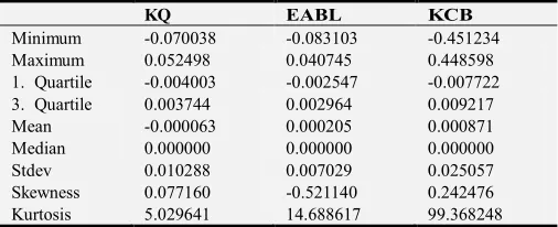
Table 1. Shows a summary statistic of the data that was used in the empirical

study.

KQ EABL KCB

Minimum -0.070038 -0.083103 -0.451234

Maximum 0.052498 0.040745 0.448598

1. Quartile -0.004003 -0.002547 -0.007722

3. Quartile 0.003744 0.002964 0.009217

Mean -0.000063 0.000205 0.000871

Median 0.000000 0.000000 0.000000

Stdev 0.010288 0.007029 0.025057

Skewness 0.077160 -0.521140 0.242476

Kurtosis 5.029641 14.688617 99.368248

The plots show that there is volatility clustering in the KQ, EABL and KCB stock as evidenced by the plot of the returns. Of importance to note is that during the period of 2007-2008, there was post elections violence that a ff e c t ed the performance of stocks unusually.

(4)

Figure 1. Plot of the stock returns.

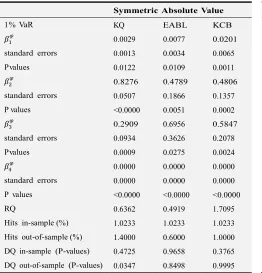
Table 2. Estimates for three CAViaR specifications at 1%.

Symmetric Absolute Value

1% VaR KQ EABL KCB

0.0029 0.0077 0.0201

standard errors 0.0013 0.0034 0.0065

P values 0.0122 0.0109 0.0011

0.8276 0.4789 0.4806

standard errors 0.0507 0.1866 0.1357

P values <0.0000 0.0051 0.0002

0.2909 0.6956 0.5847

standard errors 0.0934 0.3626 0.2078

P values 0.0009 0.0275 0.0024

0.0000 0.0000 0.0000

standard errors 0.0000 0.0000 0.0000

P values <0.0000 <0.0000 <0.0000

RQ 0.6362 0.4919 1.7095

Hits in-sample (%) 1.0233 1.0233 1.0233

Hits out-of-sample (%) 1.4000 0.6000 1.0000

DQ in-sample (P-values) 0.4725 0.9658 0.3765

DQ out-of-sample (P-values) 0.0347 0.8498 0.9995

Table 2. Continued.

asymmetric Value

1% VaR KQ EABL KCB

0.0025 0.0012 0.0101

standard errors 0.0014 0.0013 0.0040

P values 0.0368 0.1847 0.0054

0.8207 0.8857 0.7039

standard errors 0.0455 0.0853 0.1504

P values <0.0000 <0.0000 <0.0000

0.3053 0.1253 0.1665

standard errors 0.1300 0.0823 0.1632

P values 0.0094 0.0638 0.1538

0.5064 0.3633 0.7014

standard errors 0.3646 0.1967 0.6855

P values 0.0824 0.0324 0.1531

RQ 0.6320 0.4730 1.6382

Hits in-sample (%) 1.0802 1.0802 0.9665

(5)

Indirect Garch

1% VaR KQ EABL KCB

0.0001 0.0000 0.0013

standard errors 0.0000 0.0000 0.0006

P values 0.0125 0.1455 0.0193

0.8010 0.9544 0.3803

standard errors 0.0421 0.0084 0.1663

P values <0.0000 <0.0000 0.0011

0.7104 0.3068 1.2384

standard errors 0.4486 0.3156 0.6233

P values 0.0567 0.1655 0.0235

0.0000 0.0000 0.0000

standard errors 0.0000 0.0000 0.0000

P values <0.0000 <0.0000 <0.0000

RQ 0.6337 0.4942 1.7444

Hits in-sample (%) 0.9665 1.0802 1.0233

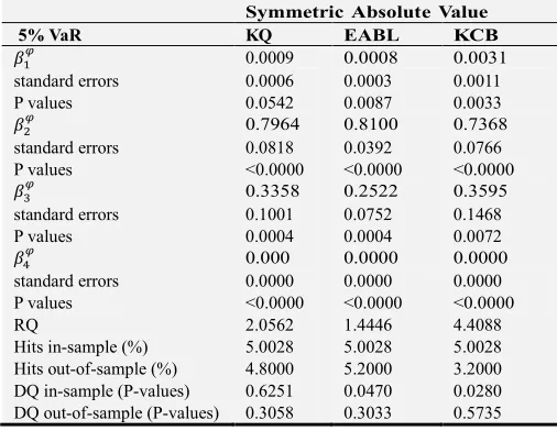
Table 3. Estimates for three CAViaR specifications at 5%.

Symmetric Absolute Value

0.0009 0.0008 0.0031

standard errors 0.0006 0.0003 0.0011

P values 0.0542 0.0087 0.0033

0.7964 0.8100 0.7368

standard errors 0.0818 0.0392 0.0766

P values <0.0000 <0.0000 <0.0000

0.3358 0.2522 0.3595

standard errors 0.1001 0.0752 0.1468

P values 0.0004 0.0004 0.0072

0.000 0.0000 0.0000

standard errors 0.0000 0.0000 0.0000

P values <0.0000 <0.0000 <0.0000

RQ 2.0562 1.4446 4.4088

Hits in-sample (%) 5.0028 5.0028 5.0028

asymmetric Value

0.0013 0.0014 0.0037

standard errors 0.0007 0.0007 0.0012

P values 0.0369 0.0258 0.0011

0.7371 0.6916 0.6876

standard errors 0.0962 0.1010 0.0530

P values <0.0000 <0.0000 <0.0000

0.2524 0.1835 0.2614

standard errors 0.1229 0.0614 0.0714

P values 0.0200 0.0014 0.0001

0.4839 0.5669 0.6064

standard errors 0.1122 0.1406 0.0729

P values <0.0000 <0.0000 <0.0000

RQ 2.0451 1.4094 4.3008

Hits in-sample (%) 5.0028 5.0028 4.9460

Indirect Garch

0.0000 0.0000 0.0001

standard errors 0.0000 0.0000 0.0001

P values 0.0295 0.0252 0.0477

0.7835 0.7622 0.6164

standard errors 0.0349 0.0528 0.1247

P values <0.0000 <0.0000 <0.0000

0.4973 0.3052 0.5397

standard errors 0.1978 0.1420 0.2325

P values 0.0060 0.0158 0.0101

0.0000 0.0000 0.0000

standard errors 0.0000 0.0000 0.0000

P values <0.0000 <0.0000 <0.0000

RQ 2.0714 1.4530 4.4863

Hits in-sample (%) 5.1165 5.1165 5.0597

Figure 2. Plot of the news impact curve for KQ stock.

(6)

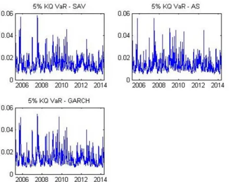
Figure 4. Plot of the 5% VaR for KQ stock.

5. Conclusion

In conclusion, the research applied the robust method of quantile regression to predict VaR using Engle & Manganelli (2004) CAViaR model applied to a sample of company from the Nairobi Securities Exchange. The class of CAViaR models which specify the evolution of quantiles over time using the autoregressive specification works well with the Kenyan Stock market data set with the asymmetric slope fitting well for the three data sets.

The findings suggest that the behavior in the tails of the distribution may be different from the rest of the distribution. The DQ out of sample tests rejects the model for this out of sample period. This suggests that there is still much to be done before achieving a satisfactory VaR model.

A non-parametric approach to estimating the parameters of the CAViaR models could be used in cases where the CAViaR model is mis specified.

References

[1] Allen, D., Singh, A., & Powell, R. “A gourmet’s delight: Caviar and the Australian stock market”. Applied Economics Letters, 19 (15), pp1493–1498, 2012.

[2] Chen, C. W., Gerlach, R., Hwang, B. B., and McAleer, M. “Forecasting value at risk using nonlinear regression quantiles and the intra-day range. International Journal of Forecasting”, 28 (3), pp557 – 574, 2012.

[3] Christoffersen, P. F. “historical simulation, value-at-risk, and expected shortfall”. (Second Edition ed., pp. 21 - 38), 2012. San Diego: Academic Press.

[4] Engle, R., and Manganelli, S. “Caviar: Conditional autoregressive value at risk by regression quantiles”, Journal of Business and economic statistics, 2004.

[5] Gourieroux, C., & Jasiak, J. “Chapter 10 - value at risk” (Vol. 1; Y. A.-S. P. HANSEN, Ed.). San Diego: North-Holland, 2010. [6] Huang, D., Yu, B., Fabozzi, F. J., & Fukushima, M.

“Caviar-based forecast for oil price risk. Energy Economics”, 31 (4), pp511 – 518, 2009.

[7] Koenker, R., & Bassett, G., Jr. “Regression quantiles.” Econometrica: journal of the Econometric Society, pp33–50, 1978.

[8] Taylor, J. W., Generating volatility forecasts from value at risk estimates.Management Science, 51 (5), pp.712–725, 2005. [9] Thupayagale, P. “Evaluation of garch-based models in

value-at-risk estimation: Evidence from emerging equity markets”. Investment Analysts Journal, pp. 13–29, 2010. [10] Wang, D. L, Huixia Judy “Estimation of high conditional

quantiles for heavy-tailed distributions”, 2012.