http://www.sciencepublishinggroup.com/j/ajtas doi: 10.11648/j.ajtas.20170605.11
ISSN: 2326-8999 (Print); ISSN: 2326-9006 (Online)
Estimating the Context Effect in a Multilevel Latent Model
with Small Sample Sizes: A Monte Carlo Simulation Study
Miao Gao
College of Education, Nanjing Normal University, Nanjing, China
Email address:
To cite this article:
Miao Gao. Estimating the Context Effect in a Multilevel Latent Model with Small Sample Sizes: A Monte Carlo Simulation Study. American Journal of Theoretical and Applied Statistics. Vol. 6, No. 5, 2017, pp. 221-227. doi: 10.11648/j.ajtas.20170605.11
Received: August 3, 2017; Accepted: August 11, 2017; Published: September 4, 2017
Abstract:
In multilevel modeling, the relationships between the criterion and predictors are investigated at different levels. Often, the level predictors are measured by aggregating the individual-level measures. However, the aggregated cluster-level predictors do not always reliably measure the cluster-cluster-level regression coefficient, and therefore the context coefficient. This study investigates an alternative approach: estimating cluster-level predictor on the latent cluster mean by using multilevel latent. A comparison is made of the accuracy of the context coefficient and standard error under a wide range of conditions. Results reveal that bias for context effect is small in multilevel latent model. Maximum likelihood (ML) estimator yields more accurate standard error estimation than robust maximum likelihood (MLR) when cluster number is small (less than 50). Very small cluster sample sizes (less than 10) should be avoided because they lack power and empirical sampling variance.Keywords:
Multilevel Latent Model, Context Effect, Parameter Estimate Accuracy, Standard Error, Power1. Introduction
Data collected in educational research are often multilevel, for example with students clustered within schools or repeated measures clustered within individuals. When data are multilevel and a predictor variable varies both within clusters and between clusters (such as individual social economic status, SES) scores varying within schools and average SES scores varying between schools), researchers are frequently interested in estimating within-cluster and between-cluster relationships of the predictor to the criterion. Often people are interested in estimating the context coefficient [1, 2, 3], that is, the difference in the regression coefficients for the between- and within-cluster relationship. Contextual analysis evaluates whether the aggregated group characteristic (L2) has an effect on the outcome variable after controlling for individual level characters (L1).
In many cases, L2 variables are based on the aggregation of L1 variables. One problematic aspect of the context effect analysis is that the observed group average obtained by aggregating individual observations may not be a very reliable measure of the unobserved group average if only a small number of L1 individuals is sampled from each L2 group [1, 4]. A few researchers explored the integration of structural
equation modeling (SEM) and multilevel modeling (MLM) to the issue of contextual analysis with the consideration of measurement error and sampling error [1, 4, 5]. The software Mplus is recommended as being particularly versatile for all forms of latent variable modeling, including the integration of SEM and MLM [1].
In the multilevel latent mean approach to estimating context effects the following equation is estimated
(
)
0
= + − + + +
ij W ij jX B jX j ij
Y γ γ X µ γ µ δ ε (1)
[4, 6]. In this equation,
µ
jX is the expected value of thepredictor scores within the j th cluster,
δ
j is a between-cluster residual, εij is a within-cluster residual,γ
0 is theintercept,
γ
W is the within-cluster regression coefficient, andB
γ
is the between-cluster regression coefficient.constructs [1]. The cluster-level averages (Xj) are estimates of the cluster-level expected values ( ) In the traditional multilevel approach to estimating context effects, Xj is used in place of
µ
jX:(
)
0 .
= + − + + +
ij W ij j B j j ij
Y γ γ X X γ X δ ε (2)
In this approach, the cluster-level averages are assumed to be measured without sampling error [3, 7]. The unreliability of the sample cluster average will lead to biased estimation of the between-cluster regression coefficient which in turn leads to bias in the context coefficient.
In the present study, the multilevel latent model is the focus and an alternative set of conditions was investigated. Specifically, the study investigated level-2 sample sizes (smaller than were investigated by Ludtke et al. [4]) and a range of intraclass correlation coefficients (ICCs) for the outcome variable. Ludtke et al. did not investigate the latter factor and the range of ICCs no doubt varies across multilevel studies. The smaller level-2 sample size was investigated because it is not unusual to find multilevel studies with the number of groups smaller than 50 [8].
In multilevel analysis, the problem with sample size is usually at the group level [9, 10, 11]. Previous research shows that a small sample size at level two leads to biased estimates of the second-level standard errors [10]; increasing the higher level sample size will improve more on power than increasing the within-cluster sample size [11]. However, in practical research, increasing the number of groups may be difficult because of the cost of bringing in new organizations and the inconvenience of finding new organizations [10, 12]. Thus seeking an alternative strategy to obtaining the accurate estimates of parameters and standard errors seems essential in the multilevel latent model.
A few researches have investigated the various estimation methods in the multilevel framework. Hox et al. [9] compared full information maximum likelihood (ML), robust maximum likelihood (MLR), and diagonally weighted least squares (DWLS) estimations in multilevel structural equation modeling. They found a clear interaction effect between number of clusters and estimation methods. They also found ML yield the most unbiased estimation than DWLS and MLR when the sample size is small. Maas and Hox [13] showed that restricted ML estimation had better coverage rates for the main fixed effects than robust estimation. Although the studies are not completely in agreement, they all conclude that the coefficients estimated are unbiased and the standard errors tend to be underestimated when the sample size is small [1, 9, 13]. In this study, MLR and ML are chosen to compare for context effect estimate. MLR is the default estimator in the multilevel model in Mplus because it offers some protection against the heterogeneity. The robust standard errors are developed to use the observed residual variance to correct the asymptotic standard errors. The likelihood function of the multilevel full ML approach in the context of SEM is defined as follows [9]:
N N
1
i i i i i
i
i 1 i 1
F log | | log(x µ) ' −(x µ)
= =
=
∑
∑
+∑
−∑
− (3)where the subscript i refers to the observed cases,
x
i refers to the variable observed for case i, and µi andi
∑
contain the population means and covariances of the variables observed for case i. Multilevel data applies in the way that clusters are as observations and individuals as variables.In this simulation study, the accuracy of context effect was examined under various conditions by using two estimators. The study varies the conditions at different levels and those conditions are within cluster sample size, number of clusters, ICC for predictor variable, ICC for criterion variable, between coefficient and context effect. The two estimators are MLR and ML.
2. Methodology
2.1. Data Generation
Simulated data were generated by using the multilevel latent model. The first step was to generate the data on the predictor. The predictor variable was decomposed into two uncorrelated components:Xij=µjX +(Xij−µjX)=µjX +RXij. The corresponding decomposition of the variance of the predictor is 2 2 2
X
X X R
σ
=τ
+σ
. Without loss of generality, the predictor variance was set equal to one. Thenτ
X2 is equal toX
ICC and 2
X R
σ
is equal to 1−ICCX. Therefore scores on thevaluable
µ
jX were generated by multiplying a standard normal variable byτ
X and scores on Rij were generated by multiplying a standard normal variable by .X
R
σ The criterion variable and its variance can be decomposed as
= +
ij jY Yij
Y
µ
R and 2= +2 2.Y
Y Y R
σ
τ σ
The criterion variancewas also set equal to one without loss of generality. Then
τ
Y2is equal to ICCY and 2
Y
R
σ
is equal to 1−ICCY.The relationship between the cluster-level means for the criterion and predictor is
µ
jY =γ
00+γ µ
01 jX +µ
0j [12]. Using standard results in regression theory,τ
Y2 =γ τ
012 2X +σ
u2. Thus once the ICCs and the between-cluster coefficient are set, the variance of the cluster-level residual is determined and can be generated by multiplying a standard normal variable by.
u
σ
The relationship between the R variables for the predictor and criterion isij ij
Y 10 X ij
R
=
γ
R
+
r
[12] and2 2 2 2
10 .
= +
Y X
R R r
σ
γ σ
σ
Once the ICCs and the within-cluster coefficient were set, the variance of the individual-level residual was determined and can be generated by multiplying a standard normal variable byσ
r.
Onceµ
jX,R
Xij,
u0j, andij
latent model yields scores on the criterion. The data were generated in Statistical Analysis System (SAS) 9.2 which was also used to call Mplus 7.0 to estimate the multilevel latent models.
2.2. Conditions
The within-cluster sample size was set to n = 5, 10, 15, or 30. A group size of 5 is usual in small-group educational research and in longitudinal research. A group size of 15 or 30 is a typical class size in school. The number of clusters was K =20 or 40. The reason we chose 20 and 40 is that a cluster sample size smaller than 50 is not unusual in multilevel empirical research, and simulation studies often focus on larger cluster sample size.
The ICCs for the predictor variable, ICC = .05, .10, .20, X and .30. The values of the ICC for the criterion variable were
=
Y
ICC .15, .2, and .3. These values are representative values found in educational research.
The between coefficients were set at γB= 7 and 5, and the context effects were γC = .3 and .1. Following the
relationship γB−γW =γC, the four combinations of γB and
C
γ were used to investigate whether the size of the between-cluster coefficient affects the accuracy of estimation of the context effect, as well as to investigate the accuracy of estimation for smaller context effects.
Overall, there were 4 2 4 3 2 2× × × × × = 384 conditions. Each condition was replicated 5000 times.
2.3. Data Analysis
For every condition, the generated data were analyzed by using the multilevel latent model to estimate the context effects with two estimators respectively in Mplus. Two estimators were MLR (maximum likelihood estimation with robust standard errors) and ML (maximum likelihood estimation). MLR is the default estimator for multilevel model in Mplus and is increasingly chosen by default in available software. MLR is assumed to offer the protection against unmodeled heterogeneity, however, Hox et al. [9] found that when number of clusters is small (less than 50) and the data follow the normality assumption, MLR does not perform as well as ML. Thus both MLR and ML were chosen for data analysis and compared the results.
To investigate accuracy of estimation, the interval estimation was estimated by using the coverage of the 95% confidence interval. Coverage, that is whether or not the CI contained the population context effect value, was coded 0-1 for each replication. Estimated coverage probability was then calculated as the mean of the dichotomous variable over the 5000 replications in each condition. Power was also investigated. Rejection of H0:
γ
C =0 against H0:γ
C≠0was coded 0-1, with a value of 1 if the CI did not contain zero (rejectH0:
γ
C =0). Estimated power was calculated asthe mean of the dichotomous variable over the 5000 replications in each condition.
Bias and sampling variability of context effect estimation
were also investigated. Bias assesses whether the expected value of the estimator of the context effect is equal to the population value of the context effect. The sampling variance of the estimator of the context effect measures how close estimates are to the expected value of the context effect. This variance was referred as the empirical sampling variance (ESV).
To investigate which factors significantly affected coverage probability and power, an analysis including seven main effects was conducted by using PROC GENMOD in SAS. Seven main factors were investigated as independent variables: γB, γC, n, K, ICC , X ICC , and estimator. Based Y
on the results of effective factors, the ML results were analyzed by using logistic regression for six main factors excluding estimator.
To investigate how the conditions in the study affected bias and empirical sampling variance (ESV), ANOVAs were conducted by using six factors as independent variables: γB,
C
γ , n, K,ICC and X ICC . Since the estimator method Y affects the standard error estimation but not the parameter itself, the ANOVA for bias and empirical sampling variance used the combined MLR and MLR results.
ESV refers to the variance of the context effect estimates. That is for qth condition of the study, ESV is
ɵ ɵ
(
)
5000 2 2 1 4999 = − =∑
i Ciq Ciq qS
γ
γ
(4)
where γɵCiq is as defined earlier and γɵCq is the mean context effect for the qth condition. To investigate how the conditions in the study affected the empirical sampling variance, the recommendation by O’Brien [14] was followed and an ANOVA was conducted using
ɵ ɵ
(
)
(
)
(
)(
)
2 2
( 1.5) .5 1
1 2
− − − −
=
− −
Ciq Cq q iq
N n S N
r
N N
γ γ
(5)
as the dependent variable, where n is the number of replicates for a condition (i.e., 5000). It can be shown that
2
.
= q q
r S Thus O’Brien’s method uses ANOVA to test hypotheses on variance.
The results of these analyses were used to calculate effect sizes. The PROC GENMOD analysis was selected to take into account the dichotomous nature of the dependent variable. To measure the relative size of the effects, the proportion of effect variance (PEV) was used.
ɵ ɵ 2 63 2 1 . = =
∑
effect effect t PEVδ
δ
(6)where 2 effect
δ is a measure of the size of the effect, ɵ
63 2
1
=
∑
effect tthe sum of
δ
ɵ2effect for the 63 effects in the ANOVA and issubsequently referred to as the total effect variance.
3. Results
3.1. Coverage Probability
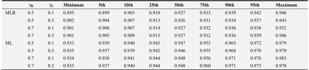
The percentiles of the coverage probability by the between coefficient and context effect using MLR and ML estimators are presented in Table 1. When using the MLR estimator, the
coverage rates range from 0.895 to 0.946 among all the conditions, which indicates the estimated standard errors of the context effect are typically negatively biased. While using the ML estimator, the coverage rates range from 0.933 to 0.983, and the median coverage rates are closer to 0.95. It shows that the ML estimator improves the estimation accuracy of standard errors and has more appropriate control of Type I error rate.
Table 1. Percentiles of Coverage Rate by Between Coefficient (γB) and Context Effect (
γ
C). Bγ γC Minimum 5th 10th 25th 50th 75th 90th 95th Maximum
MLR 0.5 0.1 0.895 0.899 0.903 0.910 0.927 0.933 0.939 0.942 0.946
0.5 0.3 0.902 0.904 0.907 0.913 0.926 0.931 0.934 0.937 0.943
0.7 0.1 0.901 0.906 0.907 0.914 0.927 0.932 0.936 0.938 0.952
0.7 0.3 0.901 0.905 0.909 0.915 0.927 0.932 0.936 0.939 0.946
ML 0.5 0.1 0.933 0.939 0.940 0.943 0.947 0.953 0.965 0.972 0.979
0.5 0.3 0.935 0.937 0.939 0.942 0.946 0.955 0.968 0.970 0.979
0.7 0.1 0.934 0.938 0.941 0.944 0.948 0.956 0.971 0.976 0.983
0.7 0.3 0.933 0.937 0.940 0.944 0.948 0.960 0.971 0.973 0.978
To further investigate which factors influence the coverage rates, the logistic regression analysis was conducted first by seven main factors: n, K, ICCX, ICCY,
B
γ
,γ
Cand estimator. Results showed the factor estimatoraccounted for the majority of the effect variance (62.2% of the total effect variance) and ML estimator showed more accurate estimation than MLR. Thus the following section focuses on the analysis of variance on ML results only.
Six factors along with their interactions were investigated for the ML coverage results by using logistic regression, and the main factors were n, K, ICCX, ICCY,
B
γ
and γC. A number of effects were significant, which is to be expected given that each cell of the design was replicated 5000 times, so the proportion of the effect variance was the focus. Cluster sample size (n) accounted for 50.6% of the total effect variance followed by ICCY for10.6% and n by K for 9.7%.
Table 2 presents mean probability coverage as a function of sample size by using the ML estimator. The effect of n on coverage probability is different than expected. Inspection of the estimated standard errors indicated that there were exceptionally large estimated standard errors for some replications and the prevalence of these large standard errors was declined as n increased, especially when K =20. The appropriate estimation occurred when within cluster sample size i10 and 15. When numbers of clusters increase from 20 to 40, the estimated standard errors tend to be more accurate at all levels of within cluster sample size. For the factorICCY,
mean coverage probability decreases from 0.955, 0.950 to 0.947 as ICCY increases from 0.15, 0.20, 0.30,
respectively. It tends to yield the most accurate estimation of standard errors when ICCY equals to 0.20.
Table 2. Mean Coverage Probability by Within Cluster Sample Size (n) and Number of Clusters (K).
n K=20 K=40
5 0.968 0.956
10 0.952 0.947
15 0.946 0.947
30 0.941 0.945
3.2. Power
Power for detecting the context effect is higher when γC
gets larger. ML estimator appropriately control type I error rates even it costs the price of power. Similar to the variance analysis of coverage, six factors along with their interactions were investigated for the ML power results by using logistic regression. The factors ICCX and γC play an important role
individually and interactively, which altogether accounted for 60.2% of the total effect variance. The within cluster sampler size (n) accounted for 9.6%.
As shown in Table 3, power increases as ICCX and γC
increase. The effect of ICCX is much larger when γC is
larger. As expected, power increases when n increases. When n increases from 5 to 30, power increases from 0.076 to 0.212. Even though the number of clusters K does not account for more than 5% of the total effect (PEV of K is 4.2%), the results showed that power increases from 0.115 to 0.181 as K increases from 20 to 40.
Table 3. Power by Context Effect (
γ
C) and Predictor Variable (ICCX).
X ICC
C
γ .05 .10 .15 .20
0.1 0.05 0.060 0.079 0.106
3.3. Bias
Results indicate that bias tends to be small in most conditions. Percentiles of bias by the between coefficient and context coefficients by using two estimators were checked. Among all conditions when using MLR, bias ranged from -0.078 to 0.151. Similar results were found when using the ML estimator. Bias ranged from -0.004 to 0.175. Median bias was 0.024 or smaller for
γ
C being 0.3, and 0.010 or smallerfor
γ
C being 0.1.Since the estimator method does not have an impact on the estimation of coefficient itself, the six-way ANOVA was conducted based on the MLR and ML-combined results which contain 10000 replications in each condition. ICCX,
n, γC along with their interactions account for 79.2% of the
total effect variance. They all have the considerate influence on the effect variance of bias.
Table 4 shows mean bias by these three factors. When
X
ICC increases, bias decreases when n is 10 or larger. Bias tends to increase as the context effect γC increases. When
C
γ is .3 and ICCX is .10 or larger, bias decreases as n
increases.
Table 4. Mean Bias by Context Effect (γC), Within Cluster Sample Size (n),
Predictor ICC (ICCX).
n
C
γ ICCX 5 10 15 30
0.1 0.05 0.008 0.031 0.038 0.013
0.1 0.10 0.024 0.025 0.015 0.010
0.1 0.15 0.016 0.009 0.005 0.007
0.1 0.20 0.006 0.004 0.002 0.004
0.3 0.05 0.006 0.089 0.106 0.051
0.3 0.10 0.075 0.072 0.042 0.014
0.3 0.15 0.045 0.023 0.013 0.006
0.3 0.20 0.015 0.008 0.004 0.003
3.4. Empirical Sampling Variance
The percentiles of the ESV of
γ
ɵC by the betweencoefficient and context effect by using MLR and ML estimators were also checked. Overall, the ESVs range form from 0.002 to 7.239 across estimators. Similar to the variance analysis of bias, the six-way ANOVA was conducted based on the MLR and ML combined results of ESV. The factors
X
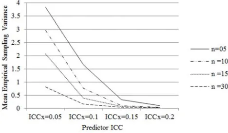
ICC , n and K accounted for 84.9% of the total effect variance for empirical sampling variance. These effects were large relative to the other effects.
For the effect of ICC , mean ESVs get smaller when X
X
ICC gets larger (Figure 1 and Figure 2). Figure 1 also shows that the mean ESV declines as n gets larger. Results in Figure 2 indicate that the mean ESV decreases when K
increases even though the number of clusters K is small (K = 20 and 40).
Figure 1. Mean Empirical Sampling Variance by Predictor ICC (ICCX)
and Within Cluster Sample Size (n).
Figure 2. Mean Empirical Sampling Variance by Number of Clusters (K) and Predictor ICC (ICCX).
4. Discussion
One notable result in this study is that ML yields more accurate parameter estimates than MLR in terms of the appropriate standard error estimation. The parameter estimates for ML and MLR are identical, so the estimates of standard errors can be compared directly. MLR, as a robust standard error estimator, performs well only when the number of clusters is large. If the data violates the distributional assumption, robust-method MLR is found to be more accurate than ML, but still requires a large sample size [9]. In the simulation study, all data are normal distributed and the sample size (especially the level-2 sample size) is relatively small. The results clearly showed that ML has more accurate parameter estimates than MLR. It is worthwhile to note that a Bayesian approach may have a great potential for estimating the latent covariate model even with a small number of groups [15, 16].
sample size increased, but the effect of cluster sample size is smaller than the number of clusters. Therefore, the findings suggest that number of groups has a positive effect on the coverage probability and the effect of group size shows an inconsistent situation. Besides, coverage probability decreases as ICCY increases, but ICCY has a smaller effect on
coverage than sample size.
Statistical power, in essence, is the probability of detecting an effect when it does exist. When the effect is smaller, the power to detect such an effect would be lower as expected. The results show that when context effect increases the power increases. The simulation study of Scherbaum and Ferreter [10] found that, at a small effect size level, the estimates of statistical power varied from approximately .05 to .28, and they considered ES=0.20 as small effects and ES=0.50 as medium effects. To investigate the power of detecting context effect (γC) in this
study, the choice of the size of context effect is relatively small. At γC = 0.1 the power ranges from 0.05 to 0.106 when ICC X
increases from .05 to .20; at γC = 0.3 the power ranges from
0.07 to 0.427.
A number of factors can influence statistical power in both single-level design and multilevel design. One of these factors is the Type I error. There is an inverse relationship between the Type I error and the power. In other words, when Type I error increases, the power decreases. This study showed that the MLR estimator consistently underestimated the Type I error given the studied conditions. The ML estimator, on the other hand, improved the accuracy of the standard error estimates. Thus the loss of power in the study is partially due to the appropriate control of Type I error by using the ML estimator.
Statistical power for multilevel models is more complicated than the single-level design since some additional factors need to be taken into account. The results show that, as expected, power increases as
γ
C,,
X
ICC n, and K increase. These results are expected and support the validity of the simulation method. Further, γB
and ICCY did not play an important role in power.
Scherbaum and Ferreter [11] argued that the intraclass correlation, the total sample size and the sample size at each level, and the inclusion of covariates all affected the computation of power. They also found that increasing the number of clusters will improve more on the power than increasing the cluster sample size. However, the results of K and n on power do not reflect this argument. Power increased much more rapidly when n increased from 5 to 10 than from 10 to a higher level. Thus it is suggested that cluster sample size should be at least 10 in terms of power in practical research.
Bias and variance are the two parameters that assess the accuracy of parameter estimation. In regard to bias, the results show that even when the number of clusters was quite small, that is between 20 and 40, bias of the context effect estimator was quite small and relatively unaffected by γB, K, and ICCY.The factors with the largest effects
on bias were ICC and X n. Bias decreased as ICC and X n
increased. The direction of each of the effects of n and
X
ICC is consistent with results in Ludtke et al. [4]. The study also indicated that bias increases as size of context effect (γC) increases. The effect of ICC and X γC on the
bias of the context effect estimator was unstable when n
was 5 but not when n was 10 or larger. Consequently, we suggest that the within-cluster sample size should be at least 10. Furthermore, ICCY, γB and K do not play an important role in the bias of the context effect estimator under the condition in the present study.
5. Conclusion
The context effect is often an important feature of multilevel data analysis. Past research has shown that, when the within-cluster sample is regarded as a sample from a larger population, the multilevel latent model, rather than the traditional multilevel model, should be used to estimate the context effect. The results suggest that the estimator ML should be used rather than MLR when the sample size is small especially the higher level sample size. ML yields more accurate estimates of the standard error so that it appropriately controls the Type I error rate. The results also suggest that bias of context effect estimation tends to be small even when the number of clusters is small. Very small within-cluster sample sizes (less than 10) should be avoided in term of power and empirical sampling variance. If the ICC for the predictor is small (.10 or less), bias is more of a problem. The fact that bias is small even when the number of clusters is small should not be taken as an argument to routinely use a small number of clusters. The number of clusters has a relatively strong effect of the sampling variance of the context effect estimator. Therefore, even an increase from 20 to 40 of cluster number is desirable in practical educational research.
Acknowledgements
The author would like to thank Dr. James Algina for his great help and the support from University of Florida and Nanjing Normal University.
References
[1] Marsh, H. W., Ludtke, O., Robitzsch, A., Trautwein, U., Asparouhov, T., Muthen, B., & Nagengast, B. (2009). Doubly-latent school contextual effects: Integrating multilevel and structural equation approaches to control measurement and sampling error. Multivariate Behavioral Research, 44(6), 764-802. [2] Raykov, T. (2007). Longitudinal analysis with regressions among random effects: A latent variable modeling approach. Structural Equation Modeling, 14(1), 146-169.
[4] Ludtke, O., Marsh, H. W., Robitzsch, A., Trautwein, U., Asparouhov, T., & Muthen, B. (2008). The multilevel latent covariate model: A new, more reliable approach to group-Level effects in contextual studies. Psychological Methods, 13(3), 203-229.
[5] Ludtke, O., Marsh, H. W., Robitzsch, A., & Trautwein, U. (2011). A 2*2 taxonomy of multilevel latent contextual models: Accuracy - bias trade-offs in full and partial error correction models. Psychological Methods, 16(4), 444-467. [6] Asparouhov, T., & Muthen, B. (2006). Constructing
covariates in multilevel regression. Mplus website. Retrieved from
http://www.statmodel.com/download/webnotes/webnote11. pdf
[7] Preacher, K. J., Zyphur, M. J., & Zhang, Z. (2010). A general multilevel SEM framework for assessing multilevel mediation. Psychological Methods, 15(3), 209-233.
[8] Lopes, P. N., Mestre, J. M., Guil, R., Kremenitzer, J. P., & Salovey, P. (2012). The Role of Knowledge and Skills for Managing Emotions in Adaptation to School Social Behavior and Misconduct in the Classroom. American Educational Research Journal, 49(4), 710-742.
[9] Hox, J. J., Maas, C. J. M., & Brinkhuis, M. J. S. (2010). The effect of estimation method and sample size in multilevel
structural equation modeling. Statistica Neerlandica, 64(2), 157-170.
[10] Maas, C. J. M., & Hox, J. J. (2005). Sufficient sample size for multilevel modeling. Methodology, 1(3), 86-92.
[11] Scherbaum, C. A., & Ferreter, J. M. (2009). Estimating statistical power and required sample sizes for organizational research using multilevel modeling. Organizational Research Methods, 12, 347-367.
[12] Snidjers, T. A. B., & Bosker, R. J. (1999). Multilevel analysis: An introduction to basic and advance multilevel modeling. London: Sage.
[13] Maas, C. J. M., & Hox, J. J. (2004). Robustness issues in multilevel regression analysis. Statistica Neerlandica, 58(2), 127-137.
[14] O’Brien, R. G. (1981). A sample test for variance effects in experimental designs. Psychological Bulletin, 89(3), 570-574. [15] Zitzmann, S., Lüdtke, O., & Robitzsch, A. (2015). A bayesian
approach to more stable estimates of group-level effects in contextual studies. Multivariate Behavioral Research, 50(6), 688-705.