Raindrop size distribution variability estimated using ensemble statistics

www.ann-geophys.net/27/555/2009/

© Author(s) 2009. This work is distributed under the Creative Commons Attribution 3.0 License.

Annales

Geophysicae

Raindrop size distribution variability estimated using ensemble

statistics

C. R. Williams and K. S. Gage

Cooperative Institute for Research in Environmental Sciences (CIRES), Univ. Colorado, Boulder, CO 80309-0216, USA Earth System Research Laboratory (ESRL), NOAA, Boulder, CO 80305, USA

Received: 18 October 2007 – Revised: 15 December 2008 – Accepted: 6 January 2009 – Published: 4 February 2009

Abstract. Before radar estimates of the raindrop size dis-tribution (DSD) can be assimilated into numerical weather prediction models, the DSD estimate must also include an uncertainty estimate. Ensemble statistics are based on using the same observations as inputs into several different mod-els with the spread in the outputs providing an uncertainty estimate. In this study, Doppler velocity spectra from col-located vertically pointing profiling radars operating at 50 and 920 MHz were the input data for 42 different DSD re-trieval models. The DSD rere-trieval models were perturbations of seven different DSD models (including exponential and gamma functions), two different inverse modeling method-ologies (convolution or deconvolution), and three different cost functions (two spectral and one moment cost functions). Two rain events near Darwin, Australia, were analyzed in this study producing 26 725 independent ensembles of mass-weighted mean raindrop diameterDm and rain rateR. The

mean and the standard deviation (indicated by the symbols hxiandσ{x}) ofDmandRwere estimated for each

ensem-ble. For small ranges ofhDmiorhRi, histograms ofσ{Dm}

andσ{R} were found to be asymmetric, which prevented Gaussian statistics from being used to describe the uncer-tainties. Therefore, 10, 50, and 90 percentiles ofσ{Dm}and

σ{R}were used to describe the uncertainties for small inter-vals ofhDmiorhRi. The smallestDmuncertainty occurred

for hDmi between 0.8 and 1.8 mm with the 90th and 50th

percentiles being less than 0.15 and 0.11 mm, which corre-spond to relative errors of less than 20% and 15%, respec-tively. The uncertainty increased for smaller and largerhDmi

values. The uncertainty ofR increased with hRi. While the 90th percentile uncertainty approached 0.6 mm h−1 _for a 2 mm h−1_{rain rate (30% relative error), the median} uncer-tainty was less than 0.15 mm h−1at the same rain rate (less

Correspondence to: C. R. Williams (christopher.williams@colorado.edu)

than 8% relative error). This study addresses retrieval error and does not attempt to quantify absolute or representative-ness errors.

Keywords. Atmospheric composition and structure (Instru-ments and techniques) – Meteorology and atmospheric dy-namics (Precipitation) – Radio science (Remote sensing)

1 Introduction

The assimilation of radar precipitation estimates into numer-ical weather prediction models is a very difficult task because the numerical models require both the precipitation estimate as well as the uncertainty of that estimate in order to blend the observations with the model. Quantifying the precipitation uncertainty from radar observations is also difficult because the uncertainty results from four types of errors: measure-ment, model, representativeness, and sampling (Bringi and Chandrasekar, 2001). Measurement errors are due to the pre-cision of the instrument. Model errors result from represent-ing observations with idealized mathematical expressions. Representativeness errors are due to time evolving changes and spatial inhomogeneity of precipitation within the sample volume during the observation dwell time. Sampling errors result from changes in precipitation between successive ob-servations.

input observations. By using the same inputs in every model, differences in the output are due to assumptions about the model precipitation physics and due to the numerical code used in the retrieval process.

Vertically pointing profiling radars have been used for over 20 years to estimate the number and size of raindrops falling directly overhead (Wakasugi et al., 1986). Three major mod-eling factors determine how the radar observations are con-verted into precipitation estimates. The first major factor is the mathematical functional shape of the raindrop size dis-tribution (DSD). Typically, there are more small raindrops within a given volume than large raindrops, which leads to the assumption that the shape of the DSD follows an ex-ponential (Waldvogel, 1974) or a gamma function (Ulbrich, 1983). By assuming a particular shape of the DSD, errors are added to the retrieved DSD because the unknown true distribution of raindrops may not follow the assumed shape. This study uses seven different DSD shape models previ-ously discussed in the literature (Waldvogel 1974; Ulbrich, 1983; Marshall and Palmer, 1948; Illingworth and Black-man, 2002; Zhang et al., 2003; Feingold and Levin, 1986).

The second major factor that contributes to the model error of precipitation estimates retrieved from vertically pointing profiling radars is the numerical inverse methodology that converts the radar observations into raindrop size distribu-tion estimates. If the DSD were known a priori, then the radar observations can be uniquely determined using radar scattering theory. This forward modeling maps the DSD into the radar domain. However, converting radar observations into the DSD domain is an inverse modeling problem and there is not a unique mapping from a given radar observation into a unique DSD. This study uses both the convolution and deconvolution numerical inverse modeling methodologies to estimate the DSD given a set of radar observations (Schafer et al., 2002; Lucas et al., 2004).

The third major factor contributing to model error is the cost function that objectively determines the “best” solution when comparing the model with the observed radar obser-vation. The most commonly used cost function involves the sum of the squared difference between the model and obser-vation. This cost function is also related to the chi-squared (χ2) statistic. Another cost function involves the absolute difference between the model and observation and is a better cost function to remove the influence of outliers. This study uses these two cost functions plus a third that compares the first three moments of the modeled and observed radar data and is a more efficient calculation than the first two cost func-tions.

Using seven DSD models, two numerical inverse model-ing methods, and three cost functions yields 42 DSD esti-mates for each radar observation. These 42 DSD estiesti-mates constitute one ensemble. The profiling radar observations from collocated 50- and 920-MHz profilers near Darwin, Australia, during two rain events are used in this study to estimate the mean mass-weighted raindrop diameter and the

rain rate. The statistics of 26 725 independent ensembles are analyzed to provide uncertainty estimates that can be applied to each precipitation estimate.

This paper has the following format. The seven different DSD models are discussed in Sect. 2. The forward model of estimating the radar reflectivity-weighted Doppler velocity spectra when given a raindrop size distribution is discussed in Sect. 3. The inverse model methodologies are presented in Sect. 4, followed by the discussion of the cost functions in Sect. 5. The profiling radar observations are discussed in Sect. 6. The ensemble statistics and conclusions are pre-sented in Sects. 7 and 8.

2 DSD models

The number and size of raindrops within a unit volume is described by the number concentration, N (D) [number m−3mm−1], also called the raindrop size distribution (DSD), whereDis the spherical equivalent diameter of each raindrop [mm]. Given the number concentration, several quantities describing the precipitation can be estimated, including the radar equivalent reflectivity factor,z[mm6m−3]. Assuming Rayleigh scattering,zis estimated using (Doviak and Zrnic, 1993)

z=

∞ Z

0

N (D)D6dD. (1)

The reflectivity factor can be expressed in log units [dBZ] using

Z=10 log₁₀(z). (2)

The rain rate,R[mm h−1], is estimated using

R= 6π 1000

∞ Z

0

N (D)D3v(D)dD (3)

where v(D)is the terminal fall speed of the raindrop ex-pressed in m s−1, and leading constants scale the rain rate so that it is expressed in mm h−1.

Another useful parameter used to describe the DSD is the mass-weighted mean drop diameter which is estimated using

Dm= ∞ R

0

N (D)D4dD

∞ R

0

N (D)D3_dD

. (4)

As can be seen from Eqs. (1) through (4), the DSD can be described in detail usingN (D)or described in general using Z,Dm, andR.

size. Therefore,N (D)is described using mathematical ex-pressions that are functions of diameter, and the following subsections describe the seven DSD models used in previous work and in this study.

2.1 Gamma distribution

The work by Ulbrich (1983) described the DSD using a mod-ified Gamma function of the form

N (D)=N0Dµexp(−3D)=N0Dµexp

−(4+µ) D Dm

(5) whereN0 is the scaling parameter [number m−3m−1−µ], µ [unitless] is the shape parameter, and 3 [mm−1] is the slope parameter which is related to the mean diameter us-ing 3=(4+µ)/Dm. While µ does influence the slope of

the distribution at large diameters,µ has a large influence on the curvature of the distribution at small diameters. When µ has negative values, the number concentration increases as the diameter decreases, and mathematically (and non-physically) has infinite number of drops with zero diameters. Conversely, whenµhas positive values the number concen-tration decreases as the diameter decreases, causing a down-ward curvature of the number concentration at small raindrop sizes.

2.2 Exponential distribution

The exponential distribution has been used in many studies to describe the DSD before Ulbrich (1983) introduced the Gamma distribution DSD model (Waldvogel, 1974). The ex-ponential DSD is a special case of the Gamma distribution DSD whenµ=0 and is expressed as

N (D)=N0exp(−3D)=N0exp

−4 D Dm

. (6)

2.3 Marshall-Palmer distribution

In the seminal work by Marshall and Palmer (1948), the DSD was described by the set of equations

NMP(D)=N0 MPexp(−3MPD) (7a)

N0 MP=8000 (7b)

3MP=4.1R−0.21 (7c)

where N0 MP is the Marshall-Palmer scale parameter and 3MPis the Marshall-Palmer slope parameter which is a func-tion of rain rate. The Marshall-Palmer (MP) distribufunc-tion is a special set of the exponential distribution DSDs constrained to have a fixed scale parameter (N0 MP=8000)and a slope parameter dependent on the rain rate. The MP distribution was developed using mid-latitude stratiform rain and it will be shown in Sect. 7 that the MP distribution is not well suited to describe the tropical rainfall data set used in this study.

2.4 Constantµgamma distribution

As previously discussed, the value ofµ in the gamma dis-tribution has a large influence on the shape of the DSD at small raindrop sizes. The work by Illingworth and Blackman (2002) suggests that radars that observe the raindrops within the Rayleigh scattering regime can not resolve the small rain-drops, and a fixed value of the shape parameter is appropri-ate for describing the DSD when using weather radars. In this study, retrievals are performed using the gamma distri-bution (Eq. 5) withµset to constant values of 2.5 and 5. A constantµreduces the Gamma function DSD (Eq. 5) to two unknowns.

2.5 Constrained gamma distribution

The gamma distribution expressed in Eq. (5) consists of 3 different variables,N0,µ, andDm. The work by Zhang et

al. (2003) and Brandes et al. (2003) suggests that a mathe-matical relationship exists betweenµ and3in the gamma distribution DSD model. While the particularµ−3 relation-ship may be precipitation regime-dependent and more work is needed to validate these relationships, this study uses the Zhang et al. (2003)µ−3relationship of

3=0.0365µ2+0.735µ+1.935. (8)

Thisµ−3relationship was converted into aµ−Dm

relation-ship using3=(4+µ)/Dmyielding

Dm=

4+µ

0.0365µ2_{+0.735µ+1.935}. (9)

2.6 Log-normal distribution

The raindrop size distribution has been described by Fein-gold and Levin (1986) using a log-normal distribution of the form

N (D)=Ntexp

−ln2

_D

Dm

2 ln2σ

(10) where Nt is the total number of drops per unit volume

[count m−3] and σ describes the width of the distribution. A unique feature of the log-normal distribution is thatN (D) approaches zero as the raindrop diameter approaches zero.

3 Radar observations of DSD

this ideal radar and atmosphere does not exist, this mathe-matical framework is useful to perform the coordinate trans-formation from the number concentration’s raindrop diam-eter domain to the radar’s raindrop fall-speed domain. The second mathematical estimate includes the finite beamwidth of a realistic radar along with the vertical motion and tur-bulence of a realistic atmosphere. These three factors con-tribute to spreading the returned power from each raindrop into several different velocity channels. Both mathematical estimates are discussed in more detail below.

3.1 Ideal radar

Assuming a perfect Doppler radar with infinitesimal beamwidth observing a uniformly distributed raindrop size distributionN (D)in a static atmosphere without any verti-cal air motion and without any turbulent motion, the modeled hydrometeor reflectivity-weighted Doppler spectral density, Shydro(v)[mm6m−3(m s−1)−1], is uniquely related toN (D) through the relation (Atlas et al., 1973)

Shydro(v)=N (D)D6dD/dv, (11)

wherevand dv are the velocity channels and velocity resolu-tion of the Doppler velocity spectrum in units of m s−1_{. The} variablesDand dD are the raindrop diameters and diame-ter resolutions corresponding tovand dv and have units of mm. The units ofShydro(v)are reflectivity per velocity chan-nel (mm6m−3)(m s−1)−1andShydro(v)has non-zero values only in the velocity channels with corresponding raindrops. While dv has the same value for each velocity channel, dD is variable and dependent on the diameterD. Through labora-tory studies, the terminal fall speed of raindrops is expressed as

vfall speed(D)=(9.65−10.3 exp(−0.6D)) _ρ

ρ0 −0.4

, (12) whereρ0andρrepresent the air densities at the ground and the level of the observation aloft, respectively (Gunn and Kinzer, 1949; Atlas et al., 1973).

3.2 Realistic radar

While Eqs. (11) and (12) describe the reflectivity-weighted Doppler velocity spectral density for an ideal radar observ-ing any possible raindrop size distributionN (D)in a static atmosphere, finite radar beamwidth and atmospheric verti-cal air motion and turbulence need to be added to the radar forward model to better represent radar observations. Both the finite radar beamwidth and atmospheric turbulence cause the observed Doppler velocity spectrum to be spread over a wider range of velocity channels. It is also important to in-clude the shift in the Doppler velocity spectrum due to the vertical air motion that shifts the raindrop terminal fall speed to the observed Doppler velocity. The spreading and shifting

ofShydro(v)is accomplished by convolvingShydro(v)by the spreading and shifting spectrum

Sair(v−ωDoppler, σair)=

1 √

2π σair

exp

"

− v−ωDoppler

2

2σ_air2

#

,(13)

whereSair(v−ωDoppler, σair)is Gaussian shaped (Gossard, 1994),ωDoppler[m s−1] is the Doppler velocity of the ambi-ent air motion defined with motions approaching the radar as positive Doppler motions consistent with the 1842 work by Christian Doppler (White, 1982), andσair[m s−1] repre-sents the spreading of the spectrum. The leading fraction in Eq. (13) normalizesSair(v−ωDoppler, σair)to unit area when integrated over all velocities so that the spectral broadening does not modify the total reflectivity ofShydro(v). The con-volution ofShydro(v)by Sair(v−ωDoppler, σair)is expressed mathematically as (Wakasuki et al., 1986)

Smodel(v)=Sair(v−ωDoppler, σair)⊗Shydro(v)+Noise, (14) where the symbol⊗represents the convolution function.

The last term in Eq. (14) is the random noise that is radar dependent and must be added to every Doppler veloc-ity channel of the Doppler spectrum. Equation (14) defines the forward model of a realistic radar and produces a realis-tic reflectivity-weighted Doppler velocity spectrum when the raindrop size distributionN (D), the air motion Doppler ve-locityωDoppler, and the spectral broadeningσair are used as inputs.

4 Numerical inverse model methodologies

While Eq. (14) constructs a modeled radar reflectivity Doppler velocity spectrum Smodel(v), the goal of DSD re-trievals is to estimate the raindrop size distribution N (D) when the radar observes a Doppler velocity spectrum Sobs(v). If the retrieved model spectrum Smodel(v) approx-imatesSobs(v)by minimizing a cost function (described in Sect. 5), thenN (D) can be estimated fromSmodel(v). One difficulty with solving this inverse problem is accounting for the convolution of Shydro(v) by the spreading and shifting spectrumSair(v−ωDoppler, σair). Two methods have been dis-cussed in the meteorological literature to account for the con-volution operation. The oldest method uses stable convolu-tion calculaconvolu-tions to estimateSmodel(v)and the newest method uses numerical deconvolution techniques to remove the in-fluence of the spreading spectrum to estimateShydro(v). In both methods,N (D)is adjusted until a cost function is min-imized. Details of both methods are described below. 4.1 Convolution method

is minimized. One advantage of this method is that calcu-latingSmodel(v)is a stable numerical operation of the for-ward model using the convolution operation. While each forward model calculation is stable, it is possible without proper numerical coding for the solution to converge to a lo-cal minimum in the cost function and not the global mini-mum. The potential of finding a local minimum versus find-ing the global minimum is a trade-off between convergence speed and searching the whole solution space. In this study, the whole solution space is searched to find the global min-imum to avoid the possibility of converging to a local mini-mum in the cost function. The convolution method has been used in many studies including Wakasugi et al. (1986, 1987); Sato et al. (1990); Currier et al. (1992); Maguire and Avery (1994); Ragopadhyaya et al. (1993, 1998, 1999); Schafer et al. (2002); and Williams (2002).

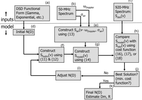
To illustrate the logic of the convolution method, Fig. 1 shows a flow diagram. The top portion (above the dashed line) of Fig. 1 shows the inputs into the convolution method which includes the DSD model, estimates of ωDoppler and σair, and the observed radar Doppler velocity spectrum of the rain. Details of estimatingωDoppler andσairfrom radar observations and the input rain spectrum are discussed in Sect. 6. The bottom portion of Fig. 1 shows the flow diagram of the convolution method. For each retrieval,ωDoppler and σairremain constant, so the spreading and shifting function Sair(v−ωDoppler, σair)needs to be calculated only once using Eq. (13) (Fig. 1e). Starting with an initialN (D)(box d), the initialShydro(v)is estimated using Eqs. (11) and (12) (Fig. 1f) and then convolved bySair(v−ωDoppler, σair)to produce an estimate ofSmodel(v)using Eq. (14) (Fig. 1g). This model spectrum is compared with the observed spectrum Sobs(v) using one of three different cost functions (Eqs. 16, 17, or 18) as discussed in Sect. 5) (Fig. 1h). If this solution does not minimize the cost function (Fig. 1j), thenN (D) is ad-justed (Fig. 1i) andShydro(v)is recalculated (Fig. 1f). The loop through Fig. 1i, f, g, h, j is repeated until the cost func-tion is minimized. After finding the best solufunc-tion,N (D)and estimates ofR andDmusing Eqs. (3) and (4) (Fig. 1k) are

saved for future analysis. The flow diagram is repeated us-ing the same radar observations but different DSD functional shape (described in Sect. 2) to yield 7 solutions for each cost function.

4.2 Deconvolution method

While the convolution method applies a spreading function to the ideal radar spectrum Shydro(v) to estimate a realis-tic radar spectrum Smodel(v) which is then compared with the observed spectrum Sobs(v), the deconvolution method applies a “de-spreading” function to the observed spectrum Sobs(v)to estimate a deconvolved spectrumSdeconv(v)which is then compared with the model spectrum from an ideal radarShydro(v). The new deconvolved spectrum is expressed

Fig. 1. Convolution method flow diagram.

as

Sdeconv(v)=Sair(v−ωDoppler, σair)⊕Sobs(v) (15) whereSobs(v)is the observed Doppler velocity spectrum and the symbol ⊕ indicates the deconvolution operation. One major difficulty with numerical deconvolution operations is that the noise in the observed spectrum can be amplified, which could lead to unstable retrievals and unrealistic solu-tions. Studies by Lucas et al. (2004) and Schafer et al. (2002) provide two examples of performing stable deconvolution routines.

Figure 2 shows a flow diagram of the deconvolution method. The top portion (above the dashed line) of Fig. 2 shows the inputs into the deconvolution method which are the same inputs as for the convolution method, and the bot-tom portion shows the flow diagram of the deconvolution method. Since for each retrieval,ωDoppler,σair, andSobs(v) remain constant,Sdeconv(v)needs to be estimated only once (see Fig. 2e and g). The iterative procedure starts with an initial estimate ofN (D)(Fig. 2d) which is used to estimate Shydro(v)(Fig. 2f), and then compared withSdeconv(v)using one of three different cost functions (16), (17), or (18) as dis-cussed in Sect. 5) (Fig. 2h). If this solution does not minimize the cost function (Fig. 2j), thenN (D)is adjusted (Fig. 2i) and Shydro(v)is recalculated (Fig. 2f). The loop through Fig. 2i, f, h, j is repeated until the cost function is minimized. After finding the best solution,N (D)and estimates ofR andDm

using Eqs. (3) and (4) (Fig. 2k) are saved for future analysis.

5 Cost functions

Fig. 2. Deconvolution method flow diagram.

the spectra. While the spectral cost functions produce model spectra that better represent the observed spectra, the mo-ment cost function is computationally faster. All three cost functions are described below.

5.1 Spectral two-norm cost function

In this study, the spectral two-norm cost function is defined as the sum of the squared difference between the modeled and observed spectra at each velocity channel and is ex-pressed as

Jkspectrak= X

i

(Sobs(vi)−Smodel(vi))2 (16)

wherei represents only the velocity channels with spectral values larger than the noise level. The value of Jkspectrak

is similar to a χ2 estimate used by Sato et al. (1990) and Schafer et al. (2002).

5.2 Spectral one-norm cost function

The spectral one-norm cost function is defined as the sum of the absolute difference between the modeled and observed spectra at each velocity channel and is expressed as

J|spectra|= X

i

|Sobs(vi)−Smodel(vi)|. (17)

The numerical benefit of the one-norm cost function over the two-norm cost function is that outliers between the model and observation contribute less to the one-norm cost func-tion. Thus, the one-norm cost function is a more robust cost function than the two-norm cost function (Aster et al., 2005). 5.3 Moment cost function

While the spectral cost functions involve every spectral point above the noise level, the moment cost function uses only the

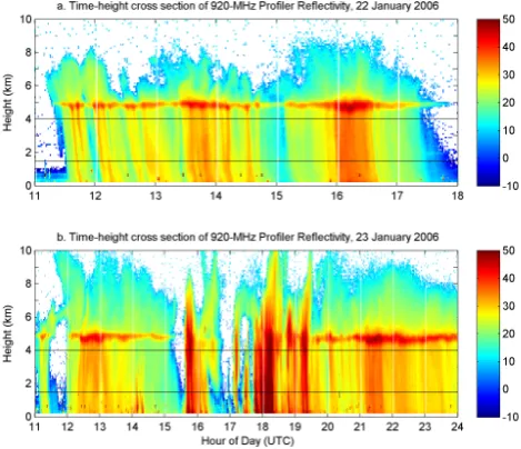
Fig. 3. Time-height cross section of radar reflectivity from the

ver-tically pointing 920-MHz profiler for (a) 22 January and (b) 23 Jan-uary 2006 during TWPICE. The lines at 1.5 and 4.0 km indicate the altitude range of DSD retrievals used in this study.

first three moments of the modeled and observed spectra and is expressed as

Jmoment=

|Zobs−Zmodel|

Zobs

+|hVobsi − hVmodeli| hVobsi

+

σ_Vobs−σ_Vmodel

σVobs

(18)

where Zobs and Zmodel are the reflectivity [dBZ] (zeroth moment expressed in dBZ), hVobsi and hVmodeli are the reflectivity-weighted mean Doppler velocity [m s−1] (first moment), andσVobs andσVmodel are the reflectivity-weighted Doppler velocity standard deviation [m s−1] (square root of the second moment) for the observed and modeled spectra, respectively. LettingS(v)denote either the observed or mod-eled spectrum, the reflectivity in units mm6m−3_{is estimated} using

z=

∞ Z

−∞

S(v)dv (19)

and can be expressed in dBZ units using Eq. (2). The reflectivity-weighted mean Doppler velocity is estimated us-ing (Williams, 2002)

hVi =

∞ R

−∞

vS(v)dv

∞ R

−∞

S(v)dv

10 8 6 4 2 0 2 4 6 8 10 12 14 0

1 2 3 4 5 6 7 8 9 10

(Upward) Doppler Velocity (ms-1) (Downward)

Altitude (km)

1 mm 3 mm 6 mm a. 50-MHz Profiler Spectral Density, 20:04 UTC

10 8 6 4 2 0 2 4 6 8 10 12 14 (Upward) Doppler Velocity (ms-1) (Downward)

1 mm 3 mm 6 mm b. 920-MHz Profiler Spectral Density, 20:04 UTC

0 20 40 60 (dBZ) c. Reflectivity

-20 -10 0 10 20 30 40 dBZ/ms-1

Air Motion Precipitation

Fig. 4. Simultaneous vertical profiles of reflectivity-weighted Doppler velocity spectral density [units of dBZ (m s−1)−1] on 23 January 2006 at 20:04 UTC for (a) the 50-MHz profiler and (b) the 920-MHz profiler. The ambient air motion is estimated from the Bragg scattering component in the 50-MHz profiler spectra (indicated in panel a). The first and second moments of the Bragg scattering component are indicated with asterisks and horizontal lines (ωDopper±σair)on the 920-MHz profiler spectra in (b). The DSD is estimated from the Rayleigh

scattering component of the 920-MHz profiler spectra shown in (b). The solid black lines labeled “1 mm”, “3 mm”, and “6 mm” indicate the air density adjusted terminal fall speeds of raindrops with diameters of 1, 3, and 6 mm, respectively.

And the reflectivity-weighted Doppler velocity standard de-viation is estimated using (Williams, 2002)

σV = 

   

∞ R

−∞

(v− hVi)2S(v)dv

∞ R

−∞

S(v)dv



   

1/2

. (21)

6 Radar observations during TWPICE

Vertically pointing profiling radar observations were col-lected in January and February 2006 during the Tropical Warm Pool – International Cloud Experiment (TWP-ICE) around Darwin, Australia. The experiment provided both remote sensing observations and aircraft in-situ measure-ments within anvil clouds which are needed to verify the microphysical properties inferred by ground-based remote sensing instruments. For this study, the Doppler velocity spectra collected by the collocated 50-MHz and 920-MHz profiling radars were used to estimate the vertical air mo-tion and the vertical profile of rain drop size distribumo-tions (DSDs). The long wavelength 50-MHz profiler observations are used to estimate the vertical Doppler motionωDopplerand the turbulent broadeningσair as the precipitation passed di-rectly over the profiler site. The shorter wavelength 920-MHz profiler observations provided the observed reflectivity-weighted Doppler velocity spectraSobs(v)used to estimate the DSD.

The time-height cross sections of reflectivity for the two rain events on 22 and 23 January 2006 used in this study are shown in Fig. 3. Both rain events had radar brightband sig-natures near 4.5 km indicative of stratiform rain. Near 15:50 and 18:20 UTC on 23 January (Fig. 3b), the reflectivity struc-ture did not contain a brightband as convective rain elements passed over the profiler site.

Examples of reflectivity-weighted Doppler velocity spec-tra observed by the two profilers while precipitation was di-rectly over the profiler site on 23 January 2006 at 20:04 UTC are shown in Fig. 4. Figure 4a was derived from the 50-MHz profiler and Fig. 4b and c were derived from the 920-MHz profiler. The colored panels in Fig. 4a and b show the reflectivity-weighted Doppler velocity spectral density S50−MHz(v) andS920−MHz(v)=Sobs(v)in units of 10 log10 ((mm6m−3)/(m s−1)) at each range gate. The logarithmic scale is used to aid in visualizing data that spans six orders of magnitude. The 920-MHz profiler reflectivity is shown in Fig. 4c and has units of dBZ.

0 10 20 30 40 50 0

0.5 1 1.5 2 2.5 3 3.5 4 4.5

Reflectivity (dBZ)

Altitude (km)

a. Reflectivity

0 1 2 3

0 0.5 1 1.5 2 2.5 3 3.5 4 4.5

Mean Drop Size, D

m (mm)

b. Mean Drop Size, D_m

0 1 2 3 4 5

0 0.5 1 1.5 2 2.5 3 3.5 4 4.5

Rain Rate (mm hour-1)

c. Rain Rate, day: 022, 13:55 UTC

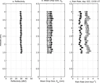
Fig. 5. Retrieved (a) reflectivity, (b) mean diameterDm, and (c) rain rate for each of the 42 DSD retrievals and at each of the 25 range gates

for 22 January 2006 at 13:55 UTC. The Marshall-Palmer (MP) DSD model retrievals are shown with circles and all other DSD models are shown with pluses. The MP solutions are over-constrained for this data set and produceDmandRthat are not consistent with the other

retrievals. MP DSD models are not used in any of the ensemble statistics.

The 50- and 920-MHz profilers operated with a coordi-nated scan strategy so that both radars were observing verti-cally for the first 45 s of every minute. The first valid range gate for the 50-MHz profiler was 1.5 km above the ground and each range gate was separated by 315 m. The 920-MHz profiler operated with 105 m range gate spacing, and the 25 range gates between 1.5 and 4 km were used in this study, which is high enough to have valid 50-MHz profiler vertical air motion estimates (1.5 km) and low enough to avoid the radar brightband (4.5 km). To account for the different verti-cal resolution of the two profilers, the 50-MHz profiler ver-tical air motion estimates at 315 m verver-tical resolution were interpolated to the 920-MHz profiler 105 m resolution. Sys-tem parameters for both profilers are listed in Table 1.

7 Ensemble statistics

For each simultaneous 50- and 920-MHz radar observation, 42 different raindrop size distributions (DSDs) were esti-mated at each of the 25 range gates between 1.5 and 4 km.

These 42 DSD estimates constitute one ensemble and were formed using seven different DSD models (see Sect. 2), two different numerical inverse model methodologies (see Sect. 4), and three different cost functions (see Sect. 5). In this study, all ensembles are studied independently of alti-tude, time, and rain regime to evaluate the statistical proper-ties of the ensemble retrieval methodology.

7.1 Filtering outliers

0 0.5 1 1.5 2 2.5 3 3.5 4 0 / 0%

300 / 10% 1500 / 50% 2700 / 90% 3000 / 100%

Mean Diameter, <D

m> (mm)

CNT & % Accum.

a. Histogram and Percent Accumulation of mean Diameter, <D

m>, Total CNT: 26725

Histogram % Accumulation Tot. cnt: 26725 10%: 0.90 mm 50%: 1.50 mm 90%: 2.10 mm

0 0.05 0.1 0.15 0.2 0.25 0.3 0.35 0.4

0 / 0% 30 / 10% 150 / 50% 270 / 90% 300 / 100%

Standard Deviation of D

m for each Ensemble, σ {Dm} (mm)

CNT & % Accum.

b. Histogram and Percent Accumulation, σ {D

m} for <Dm> between 1.45 & 1.55 mm

Histogram % Accumulation Tot. cnt: 2474 10%: 0.05 mm 50%: 0.10 mm 90%: 0.14 mm

Fig. 6. Panel (a) shows the histogram ofhDmioccurrence for all 26 725 ensembles as a function of retrievedhDmi(solid line) and the

percent accumulation from 0 to 100% (dashed line). Panel (b) shows the histogram ofσ{Dm}for the small range of 1.45<hDmi<1.55 mm.

Panel (b) also shows the percent accumulation from 0 to 100% of these 2474 ensembles in this sub-set. The values of the 10th, 50th, and 90th percentiles are indicated in the two panels.

Table 1. Operating parameters of the Darwin 50- and 920-MHz profilers (V is vertical, E is east, and N is north).

Parameter 50-MHz Profiler 920-MHz Profiler

Scan sequence V(45 s), E(15 s), V(45 s), N(15 s) V(45 s), E(15 s), V(45 s), N(15 s) Height resolution 315 m 105 m

Height coverage 1.5–20 km 200 m–12 km

Beamwidth 3◦ 9◦

other DSD Models, and the MP rain rateR is consistently greater than the other DSD Models.

These biases occurred with nearly every profile during the two rain events and theDmbias for each DSD estimate

rel-ative to the ensemble mean is shown in Table 2. The 42 DSD estimates are shown in Table 2 with the seven rows corresponding to the DSD models and the six columns corre-sponding to the two numerical model methods and the three cost functions. The bias for each DSD estimate is defined us-ing allnobservations from both rain events and determined using

Bias=1 n

n X

i

Destimate_m,i −hDmii

(22) whereD_m,iestimate is a particular DSD estimate andhDmii is

the ensemble mean using all 42 DSD estimates for eachit h observation. The MP DSD model Dm is biased low

rela-tive to the ensemble mean for all six numerical methods by at least 0.4 mm. ThisDmunderestimate leads to a rain rate

over estimate. TheDmbias indicates that the constraints of

0 1 2 3 4 5 6 7 8 9 10 0 / 0%

250 / 10% 1250 / 50% 2250 / 90% 2500 / 100%

Mean Rain Rate, <R> (mm hour-1)

CNT & % Accum.

a. Histogram and Percent Accumulation of mean Rain Rate, <R>, Total CNT: 26725

Histogram % Accumulation Tot. cnt: 26725 10%: 0.10 mm/hr 50%: 0.80 mm/hr 90%: 4.80 mm/hr

0 0.1 0.2 0.3 0.4 0.5 0.6 0.7 0.8 0.9 1

0 / 0% 10 / 10% 50 / 50% 90 / 90% 100 / 100%

Standard Deviation of R for each Ensemble, _σ {R} (mm hour-1)

CNT & % Accum.

b. Histogram and Percent Accumulation, σ {R} for <R> between 1.45 & 1.55 mm hour-1

Histogram % Accumulation Tot. cnt: 562 10%: 0.04 mm/hr 50%: 0.08 mm/hr 90%: 0.32 mm/hr

Fig. 7. Panel (a) shows the histogram ofhRioccurrence for all 26 725 ensembles as a function of retrievedhRi(solid line) and the percent accumulation from 0 to 100% (dashed line). Panel (b) shows the histogram ofσ{R}for the small range of 1.45<hRi<1.55 mm h−1. Panel (b) also shows the percent accumulation from 0 to 100% of these 562 ensembles in this sub-set. The values of the 10th, 50th, and 90th percentiles are indicated in the two panels.

database, leaving a maximum number of 36 members in each ensemble.

It is understood that with the ensemble modeling paradigm, not all models produce realistic results for every situation. Therefore, the remaining 36 mean raindrop diam-eterDmand 36 rain rateRestimates for each ensemble were

screened for outliers using a two-step filter. First, the me-dian and standard deviation ofDm andR (D˜m,R,˜ σ{Dm},

andσ{R})were estimated for each ensemble of 36 DSD esti-mates. The second step removed all DSD estimates that were either outside the bounds ofD˜m±2σ{Dm}or R˜ ±2σ{R},

or greater thanR˜+2R. After this two-step filter, all ensem-˜ bles with less than 28 members were eliminated from the database, leaving a total of 26 725 independent ensembles each with at least 28 DSD estimates.

7.2 Statistical measures of the ensembles

After each ensemble was filtered to remove outlier DSD estimates, the mean and standard deviation of Dm and R

were estimated for each ensemble (hDmi,σ{Dm},hRi, and

σ{R}). The top panel of Fig. 6 shows the histogram ofhDmi

and the percent accumulation for all 26 725 ensembles.

Vi-sual inspection suggests that thehDmi histogram is

quasi-symmetric and the uniform distribution of the 10, 50 and 90 percentiles with values of 0.9, 1.5, and 2.1 mm supports a quasi-symmetric histogram. The bottom panel of Fig. 6 shows the histogram and percent accumulation of σ{Dm}

for a sub-set of 2474 ensembles that have hDmi between

1.45 and 1.55 mm. While visually, theσ{Dm}histogram

ap-pears asymmetric with more larger values than smaller val-ues, quantitatively, the 10th, 50th, and 90th percentile values are nearly uniformly distributed with values of 0.05, 0.10, and 0.14 mm, suggesting a quasi-symmetric distribution.

Table 2. Bias ofDmfor each DSD estimate relative to the ensemble mean (see Eq. 22). Each row corresponds to a DSD model (described

in Sect. 2) with the model equation shown in the parentheses. Each column corresponds to a numerical inverse method (described in Sect. 4) and a cost function (described in Sect. 5).

DSD model (Eq. #) Convolution method Deconvolution method

Jkspectrak J|spectra| Jmoment Jkspectrak J|spectra| Jmoment

Gamma (5) 0.031 0.033 0.029 −0.003 0.005 0.045 Exponential (6) −0.103 −0.093 −0.056 −0.124 −0.123 −0.039 Marshall-Palmer (7) −0.485 −0.527 −0.467 −0.516 −0.560 −0.527 Gamma withµ=2.5 (5) 0.060 0.050 0.061 0.038 0.021 0.072 Gamma withµ=5 (5) 0.128 0.112 0.138 0.100 0.082 0.148 Constrained Gamma (9) 0.031 0.034 0.021 0.025 0.029 0.008 Log-Normal (10) 0.152 0.144 0.078 0.133 0.125 0.108

interval ofhRi. Therefore, the uncertainty of hRi is quan-tified using the 10th, 50th, and 90th percentiles ofσ{R}for small intervals ofhRi. For consistency in the analysis, un-certainties in hDmi will also be quantified using the 10th,

50th, and 90th percentiles ofσ{Dm}for each small interval

ofhDmi, even though the frequency distributions are

quasi-Gaussian in shape.

7.3 Uncertainties for small ranges ofDmand R

Due to the non-linear and non-Gaussian distribution of en-semble statistics discussed in the previous section, estimat-ing the uncertainty inDmandRrequires estimating the 10th,

50th, and 90th percentiles ofσ{Dm}andσ{R}for small

in-tervals ofhDmiandhRi. In particular, for each small

inter-val ofhDmiorhRi, the corresponding population ofσ{Dm}

andσ{R}are sorted to estimate the 10th, 50th, and 90th per-centiles ofσ{Dm}andσ{R}. Figure 8 shows the

10th-to-90th percentile ranges plus the 50th percentile value forhDmi

ranging from 0.4 to 2.7 mm in 0.1 mm intervals (top panel) and forhRi ranging from 0.0 to 2.3 mm h−1in 0.1 mm h−1 intervals (bottom panel). The 50th percentile is shown for eachhDmiandhRiwith the horizontal bar in both panels.

The smallestDmuncertainty occurs forhDmibetween 0.8

and 1.8 mm and the 90th percentile is less than 0.15 mm and the median value is less than 0.11 mm. The uncertainty in-creases for small and largerhDmi values, which is

consis-tent with the simulations performed by Schafer et al. (2002). The uncertainty of R increases with hRi. While the 90th percentile uncertainty approaches 0.6 mm h−1_{for 2 mm h}−1 rain rate (30% relative error), the median uncertainty is less than 0.15 mm h−1_{at this rain rate (less than 8% relative} er-ror). The non-uniform spacing between the rain rate 10th, 50th and 90th percentiles highlights the non-linear rain rate error between the different retrieval methodologies.

8 Conclusions

Before radar estimates of the raindrop size distribution (DSD) can be assimilated into numerical weather predic-tion models, the retrieved DSD must include both the esti-mated precipitation parameter (i.e., reflectivity, mean mass-weighted diameter, rain rate) and an estimate of the uncer-tainty. The ensemble methodology enables the DSD un-certainty to be estimated by measuring the spread in DSD retrievals that use the same observations as inputs but use different retrieval methodologies to estimate the DSD. The DSD retrieval methodologies are dependent on how the DSD is modeled, how the numerical inversion method is imple-mented, and how the cost function is defined to determine the “best” solution.

In this study, seven different DSD models were used to mathematically describe the raindrop size distribution and included a Gamma distribution, an exponential distribution, a Marshall-Palmer distribution, constant µ=2.5 and µ=5 Gamma distributions, a Gamma distribution constrained us-ing aµ−Dmrelationship, and a log-normal distribution. The

convolution method and deconvolution method were the two numerical inversion methods used in this study. And, three cost functions were used to compare the observations and models and included two point-by-point cost functions and one moment cost function. For each set of radar observa-tions, 42 different DSD estimates were generated to form one ensemble. The retrieved DSDs were parameterized by the reflectivity, mass-weighted mean diameterDm, and rain

rateR.

By comparing the 42 DSD parameters of reflectivity,Dm,

andR at each range gate for every profile during two rain events, it was determined that the Marshall-Palmer (MP) DSD model produced DSD parameters withDm too small

0 0.5 1 1.5 2 2.5 3 0.0

0.2 0.4 0.6 0.8

Mean Diameter, <D_m> (mm)

σ

{D

m

} (mm)

a. Median and 10th-to-90th Percentiles of σ {D

m} for each <Dm> +/- 0.05 mm

0 0.5 1 1.5 2 2.5 3

0.0 0.2 0.4 0.6

Mean Rain Rate, <R> (mm hour-1)

σ

{R} (mm hr

-1 )

b. Median and 10th-to-90th Percentiles of σ {R} for each <R> +/- 0.05 mm hour-1

Fig. 8. Panel (a) shows the 10th-to-90th percentile ranges ofσ{Dm}for 0.1 mm intervals ofhDmi. The median value for eachhDmiinterval

is shown with a horizontal line. Panel (b) shows the 10th-to-90th percentile ranges ofσ{R}for 0.1 mm h−1intervals ofhRialong with the median value shown with a horizontal line.

were independent of range gate suggesting that the MP DSD model, which was developed using mid-latitude stratiform rain events, was not appropriate for these tropical rain events. Therefore, the MP DSD model runs were eliminated from the ensemble database. After removing outliers from individual ensembles, 26 725 ensembles were used in this study with at least 28 DSD estimates in each independent ensemble.

In order to estimate the uncertainty of theDmandR

esti-mates, small intervals of meanDm and meanR (hDmi and hRi) were identified, and the spread in the corresponding σ{Dm}andσ{R}were studied in detail. The histograms of

σ{Dm}andσ{R}were not symmetric which prevented the

use of Gaussian statistics (estimates of mean and standard deviation) to describe the histograms and to describe the un-certainties ofDmandR. Therefore, the 10th, 50th, and 90th

percentiles ofσ{Dm} andσ{R}were used to describe the

uncertainty ofDmandRfor small intervals ofDmandR.

The smallest Dm uncertainty occurs for hDmi between

0.8 and 1.8 mm and the 90th percentile is less than 0.15 mm which corresponds to a relative error of less than 20%. The median value ofσ{Dm}was less than 0.11 mm and

corre-sponds to a relative error of less than 15%. The uncer-tainty increases for smaller and larger hDmi values. The

uncertainty ofR increases with hRi. While the 90t h per-centile uncertainty approaches 0.6 mm h−1for 2 mm h−1rain rate (30% relative error), the median uncertainty is less than 0.15 mm h−1at this rain rate (less than 8% relative error). Acknowledgements. This work was supported in part by the

NASA Tropical Rainfall Measuring Mission (TRMM) and Pre-cipitation Measurement Mission (PMM) programs (award number NNX07AN32G), and in part by NOAA’s contribution toward the NASA PMM program. The Darwin 50-MHz profiler is owned and operated by the Australian Bureau of Meteorology (BOM). The Darwin 920-MHz profiler was owned by NOAA and is maintained and operated by BOM.

References

Aster, R. C., Borchers, B., and Thurber, C. H.: Parameter Estima-tion and Inverse Problems, Elsevier Academic Press, London, UK, 301 pp., 2005.

Atlas, D., Srivastava, R. S., and Sekhon, R. S.: Doppler radar char-acteristics of precipitation at vertical incidence, Rev. Geophys., 11, 1–35, 1973.

Brandes, E. A., Zhang, G., Vivekanandan, J.: An evaluation of a drop distribution–based polarimetric radar rainfall estimator, J. Appl. Meteorol., 42, 652–660, 2003.

Bringi, V. N. and Chandrasekar, V.: Polarimetric Doppler Weather Radar, Cambridge University Press, 636 pp., 2001.

Currier, P. E., Avery, S. K., Balsley, B. B., Gage, K. S., and Ecklund, W. L.: Combined use of 50 MHz and 915 MHz wind profilers in the estimation of raindrop size distributions, Geophys. Res. Lett., 19, 1017–1020, 1992.

Doviak, R. J. and Zrnic, D. S.: Doppler Radar & Weather Observa-tions, Academic Press, 562 pp., 2nd edn., 1993.

Feingold, G. and Levin, Z.: The lognormal fit to raindrop spectra from frontal convective clouds in Israel, J. Appl. Meteorol., 25, 1346–1364, 1986.

Gossard, E. E.: Measurement of cloud droplet spectra by Doppler radar, J. Atmos. Oceanic Technol., 11, 712–726, 1994.

Gunn, R., and Kinzer, G. D.: The terminal velocity of fall for water droplets in stagnant air, J. Meteor., 6, 243–248, 1949.

Illingworth, A. J. and Blackman, T. M.: The need to represent rain-drop size spectra as normalized gamma distributions for the inter-pretation of polarization radar observations, J. Appl. Meteorol., 41, 286–297, 2002.

Lucas, C., MacKinnon, A. D., Vincent, R. A., and May, P. T.: Rain-drop size distribution retrievals from a VHF boundary layer pro-filer, J. Atmos. Oceanic Technol., 21, 45–60, 2004.

Maguire II, W. B. and Avery, S. K.: Retrieval of raindrop size dis-tributions using two Doppler wind profilers: Model sensitivity testing, J. Appl. Meteorol., 33, 1623–1635, 1994.

Marshall, J. S. and Palmer, W. M. K.: The distribution of raindrops with size, J. Meteor., 5, 165–166, 1948.

Rajopadhyaya, D. K., May, P. T., and Vincent, R. A.: A general approach to the retrieval of raindrop size distributions from wind profiler Doppler spectra: Modeling results, J. Atmos. Oceanic Technol., 10, 710–717, 1993.

Rajopadhyaya, D. K., May, P. T., Cifelli, R. C., Avery, S. K., Willams, C. R., Ecklund, W. L., and Gage, K. S.: The ef-fect of vertical air motions on rain rates and median volume di-ameter determined from combined UHF and VHF wind profiler measurements and comparisons with rain gauge measurements, J. Atmos. Oceanic Technol., 15, 1306–1319, 1998.

Rajopadhyaya, D. K., Avery, S. K., May, P. T., and Cifelli, R. C.: Comparison of precipitation estimation using single- and dual-frequency wind profilers: Simulations and experimental results, J. Atmos. Oceanic Technol., 16, 165–173, 1999.

Sato, T., Hiroshi, D., Iwai, H., Kimura, I., Fukao, S., Yamamoto, M., Tsuda, T., and Kato, S.: Computer processing for deriv-ing drop-size distributions and vertical air velocities from VHF Doppler radar spectra, Radio Sci., 25, 961–973, 1990.

Schafer, R., Avery, S. K., May, P., Rajopadhyaya, D., and Williams, C. R.: Estimation of rainfall drop size distributions from dual-frequency wind profiler spectra using deconvolution and a non-linear least square fitting technique, J. Atmos. Oceanic Technol., 19, 864–874, 2002.

Ulbrich, C. W.: Natural variations in the analytical form of the rain-drop size distribution, J. Appl. Meteorol., 22, 1764–1775, 1983. Wakasugi, K., Mizutani, A., Matsuo, M., Fukao, S., and Kato, S.: A

direct method for deriving drop-size distribution and vertical air velocities from VHF Doppler radar spectra, J. Atmos. Oceanic Technol., 3, 623–629, 1986.

Wakasugi, K., Mizutani, A., Matsuo, M., Fukao, S., and Kato, S.: Further discussion on deriving drop-size distribution and vertical air velocities directly from VHF Doppler radar spectra, J. Atmos. Oceanic Technol., 4, 170–179, 1987.

Waldvogel, A.: TheN0jump of raindrop spectra, J. Atmos. Sci.,

31, 1067–1078, 1974.

White, D.: Johann Christian Doppler and his effect – A Brief his-tory, Ultrasound Med. Biol., 8, 583–591, 1982.

Williams, C. R.: Simultaneous ambient air motion and raindrop size distributions retrieved from UHF vertical incident profiler ob-servations, Radio Sci., 37(2), 1024, doi:10.1029/2000RS002603, 2002.