Landscape-scale changes in forest structure and functional traits along an Andes-to-Amazon elevation gradient

www.biogeosciences.net/11/843/2014/ doi:10.5194/bg-11-843-2014

© Author(s) 2014. CC Attribution 3.0 License.

Biogeosciences

Landscape-scale changes in forest structure and functional traits

along an Andes-to-Amazon elevation gradient

G. P. Asner1, C. B. Anderson1, R. E. Martin1, D. E. Knapp1, R. Tupayachi1, F. Sinca1, and Y. Malhi2 1_{Department of Global Ecology, Carnegie Institution for Science, 260 Panama Street, Stanford CA 94305, USA} 2_{School of Environment and Geography, University of Oxford, South Parks Road, Oxford OX1 3QY, UK} Correspondence to: G. P. Asner ([email protected])

Received: 17 August 2013 – Published in Biogeosciences Discuss.: 27 September 2013 Revised: 8 January 2014 – Accepted: 9 January 2014 – Published: 11 February 2014

Abstract. Elevation gradients provide opportunities to

ex-plore environmental controls on forest structure and func-tioning. We used airborne imaging spectroscopy and lidar (light detection and ranging) to quantify changes in three-dimensional forest structure and canopy functional traits in twenty 25 ha landscapes distributed along a 3300 m ele-vation gradient from lowland Amazonia to treeline in the Peruvian Andes. Elevation was positively correlated with lidar-estimated canopy gap density and understory vegeta-tion cover, and negatively related to canopy height and the vertical partitioning of vegetation in canopies. Increases in canopy gap density were tightly linked to increases in under-story plant cover, and larger gaps (20–200 m2)produced 25– 30 times the response in understory cover than did smaller gaps (< 5 m2). Vegetation NDVI and photosynthetic frac-tional cover decreased, while exposed non-photosynthetic vegetation and bare soil increased, with elevation. Scaling of gap size to gap frequency (λ)was, however, nearly con-stant along the elevation gradient. When combined with other canopy structural and functional trait information, this sug-gests near-constant canopy turnover rates from the lowlands to treeline, which occurs independent of decreasing biomass or productivity with increasing elevation. Our results provide the first landscape-scale quantification of forest structure and canopy functional traits with changing elevation, thereby im-proving our understanding of disturbance, demography and ecosystem processes in the Andes-to-Amazon corridor.

1 Introduction

Tropical elevation gradients offer natural laboratories for studies of environmental controls on forest composition, structural habitats, functional processes, and ecosystem de-velopment (Vitousek et al., 1992). Studies to date have used field-based observations to quantify elevation-related changes in nutrient cycling, productivity and a variety of plant traits (e.g., Alves et al., 2010). Results often show that species composition changes markedly with increasing ele-vation in the tropics (Silman, 2006; Lieberman et al., 1996), yet patterns of canopy functional traits and productivity have been much more variable (e.g., Vitousek et al., 1988; Raich et al., 1997; Girardin et al., 2010). Indeed, field-based eleva-tion studies report wide-ranging results that are challenging to synthesize into generalizable patterns and emergent prin-ciples (Tanner et al., 1998; Hodkinson, 2005).

While reports on elevation-based changes in functional traits vary widely in the tropics, patterns of and the processes underlying forest canopy structure such as volume, canopy layering and gap dynamics remain even less understood. Yet canopy structure expresses the outcome of, and mediates the future of, functional processes such as light use, turnover and net primary productivity, or NPP (Asner et al., 1998; Brokaw, 1985b). Structure also creates the habitat for all other forest-dwelling species (Terborgh, 1992), so a quantitative standing of canopy structural change with elevation under-pins conservation and management planning.

difficult to study, owing to rough terrain, poor road and river access, and arduous overland distances. Another problem centers on ecological scale; perhaps every study thus far pub-lished on elevation-related changes in tropical forest proper-ties has focused either on individual species or in plots no larger than a hectare. Yet habitats vary locally at any given el-evation, simply based on slope, aspect and disturbance. This hampers efforts to determine the average effects of elevation on canopy structural properties and functional processes.

Remote sensing offers to overcome the limits of field work by providing measurements of forests at larger geographic scales. However, persistent cloud cover common to tropical mountains severely limits the utility of satellite-based obser-vations (Ticehurst et al., 2004). Airborne platforms offer a solution because the measurements can be planned around local cloud cover dynamics. More importantly, airborne tech-niques offer far more biophysical and functional trait in-formation than do current satellite-based approaches. Forest functional traits, including light interception, foliar cover and canopy chemistry, are often reported using hyperspectral data collected with imaging spectrometers (reviews by Kokaly et al., 2009; Ustin et al., 2004). Forest canopy structure is in-creasingly being explored using airborne Light Detection and Ranging (lidar) systems (Lefsky et al., 2002; Drake et al., 2002). Combined, imaging spectroscopy and lidar represent a powerful approach, providing uniquely high data dimen-sionality required to probe the composition, structure and functioning of ecosystems (Asner et al., 2012b). However, these newer technologies have not been applied to tropical elevation gradients.

The Andes-to-Amazon corridor stretches 2000 km from Colombia to Bolivia, and from elevations of∼100 m in the Amazon lowlands to nearly 4000 m at the Andean treeline. The forest canopy is comprised of thousands of plant species arranged in communities associated with changing elevation, geology, soils and hydrological conditions (Gentry, 1988). To date, most studies of forest functional and structural patterns have focused on the Amazon lowlands, demonstrating that forest canopy height, aboveground biomass and foliar nutri-ent concnutri-entrations vary by community, soil type and geologic substrate (Quesada et al., 2012; Baker et al., 2004; Fyllas et al., 2009; Asner et al., 2010). A recent study also found that canopy gap-size frequency distributions – a quantitative expression of turnover patterns – are surprisingly constant throughout the southwestern Amazonian lowlands (Asner et al., 2013).

In comparison to the lowlands, we have little knowledge of canopy structural and functional variation along eleva-tion gradients up to the Andean treeline. Recent plot-based studies suggest that aboveground biomass decreases with increasing altitude, and NPP declines at elevations above 1500 m a.s.l. (Girardin et al., 2010; Huaraca Huasco et al., 2014; Moser et al., 2011). This occurs despite the fact that leaf area index (LAI) and photosynthetic capacity (Amax)

remain fairly constant, thus pointing to decreased energy

inputs (cloud cover) and temperature-lowering carbon uptake at higher elevations (Y. Malhi, unpublished data). Decreas-ing biomass paralleled by decreasDecreas-ing productivity also sug-gests nearly constant residence time, as reported by Girardin et al. (2014). If true, this should be reflected in near-constant patterns of canopy gap formation along elevation gradients, but this has not yet been assessed.

We quantified landscape-scale changes in forest canopy structural and functional properties from lowland Amazonia to the Andean treeline in Peru. Our assessment was carried out at an ecological scale thus far unachieved in the field – 25 ha forest landscapes in 20 unique abiotic settings de-scribed by varying elevation, climate and soils. We used the Carnegie Airborne Observatory (CAO) Airborne Taxonomic Mapping System (AToMS) to collect multi-dimensional measurements of vegetation (Asner et al., 2012b), and to answer these questions: (i) How do canopy height and the vertical partitioning of the vegetation change with elevation? (ii) Do canopy gaps co-vary with changes in canopy struc-ture along the elevation gradient? (iii) How do canopy func-tional traits such as light interception, photosynthetic and non-photosynthetic vegetation cover, and greenness change with elevation? (iv) Do structural and functional traits co-vary with one another, and if so, how does elevation affect relationships between traits? (v) Do remotely sensed canopy properties corroborate plot-based suggestions of nearly con-stant biomass turnover along an Andes-to-Amazon elevation gradient?

2 Methods

2.1 Study landscapes

2.2 Airborne data collection

The airborne data were collected in August/September 2011. CAO AToMS includes a Visible-to-shortwave Infrared (VSWIR) imaging spectrometer and a dual laser, waveform lidar (Asner et al., 2012b). These sub-systems are boresight aligned onboard a Dornier 228–202 aircraft. We collected AToMS data over each study landscape from an altitude of 2000 m a.g.l., at an average flight speed of 55–60 m s−1and a mapping swath of 1.2 km.

The VSWIR spectrometer collects data in 480 contigu-ous spectral channels spanning the 252–2648 nm wavelength range with 5 nm (full-width at half-maximum) bandwidth. It has a 34◦ _{field-of-view and an instantaneous field-of-view} of 1 mrad. At 2000 m a.g.l., the VSWIR data provided 2 m ground sampling distance, or pixel size, throughout each study landscape. The lidar has a beam divergence set to 0.5 mrad, and was operated at 200 kHz with 17◦scan half-angle from nadir, providing swath coverage similar to the VSWIR spectrometer. Because the CAO AToMS data were collected from adjacent flightlines with 50 % overlap, the li-dar point density achieved was approximately 2 shots m−2, or 8 shots per VSWIR pixel.

2.3 Data processing

Laser ranges from the lidar were combined with embedded high-resolution global positioning system-inertial measure-ment unit (GPS-IMU) data to determine the 3-D locations of laser returns, producing a “cloud” of lidar data. The lidar data cloud consists of a very large number of georeferenced point elevation estimates (cm), where elevation is relative to a reference ellipsoid (WGS 1984). To estimate canopy height above ground, lidar data points were processed to identify which laser pulses penetrated the canopy volume and reached the ground surface. We used these points to interpolate a raster digital terrain model (DTM) for the ground surface. This was achieved using a 10 m×10 m kernel passed over each flight block; the lowest elevation estimate in each ker-nel was assumed to be ground. Subsequent points were eval-uated by fitting a horizontal plane to each of the ground seed points. If the closest unclassified point was < 5.5◦and < 1.5 m higher in elevation, it was classified as ground. This process was repeated until all points within the block were evaluated. The digital surface model (DSM) was based on interpolations of all first-return points. Measurement of the vertical differ-ence between the DTM and DSM yielded a model of canopy height above ground (digital canopy model, DCM).

The vertical distribution of lidar points was processed by binning the data into volumetric pixels (voxels) at 5 m×5 m spatial and 1 m vertical resolution (Asner et al., 2008). The DTM was used to standardize the vertical datum of each voxel. Therefore, the heights of each vertical “slice” of a vegetation canopy were defined relative to the ground at the horizontal center of each voxel. After all lidar points were

binned in the volume cube, each vertical column of the cube was divided by the total number of lidar points in that col-umn, yielding the percentage of lidar points that occurred in each voxel. This approach has the advantage of decreasing our sensitivity to localized variations in canopy leaf density or tree branch characteristics, which can result in a different number of lidar returns from voxel to voxel. It is important to note that our vertical profiles are based on lidar returns, which serve as proxies for actual vertical canopy profiles (Lefsky et al., 1999; Asner et al., 2008).

The VSWIR data were radiometrically corrected to radi-ance (W sr−1m−2) using a flat-field correction, radiomet-ric calibration coefficients, and spectral calibration data col-lected in the laboratory. We created a camera model to pre-cisely describe the three-dimensional location and field-of-view of each sensor and, combined with standardized tim-ing information, for high-precision data co-registration. A smoothed best estimate of trajectory (SBET), lidar DTM, and camera model were then used to produce an image ge-ometry model and observational data containing informa-tion on exact solar and viewing geometry for each image pixel. These inputs were used to atmospherically correct the radiance imagery to apparent surface reflectance using the ACORN-5 model (Imspec LLC, Glendale, CA USA). To im-prove aerosol corrections in ACORN-5, we iteratively ran the model with different visibilities until the reflectance at 420 nm (which is almost constant for vegetated pixels) was 1 %. The reflectance data were then corrected for cross-track brightness gradients using a bidirectional reflectance distri-bution function (BRDF) model (Colgan et al., 2012). The imagery was then geo-orthorectified to the lidar DCM. In ad-dition, the precise positioning of the lidar-to-VSWIR data al-lowed for automated masking of pixels shaded by neighbor-ing canopies and branches, as well as water bodies (Fig. A1) (Asner et al., 2007).

2.4 Analysis

canopy height; a lowP :Hratio indicates a groundward ten-dency of foliar distribution.

We mapped and analyzed gaps in the forest canopy by ap-plying a definition similar to Brokaw’s (1982) definition to the DCM results whereby all gaps down to 2 m above ground level were mapped and their areas quantified. We also quan-tified the gap-size frequency distribution using the Zeta dis-tribution, which is a discrete power-law probability density (Kellner and Asner, 2009). For the Zeta distribution with pa-rameterλ, the probability that gap size takes the integer value kis

f (k)= k

−λ

ξ(λ), (1)

where the denominator is the Riemann zeta function, and is undefined forλ=1. This distribution is sometimes called the “discrete Pareto distribution”, and is appropriate for model-ing the size-frequency of canopy gaps (Clauset et al., 2007; Fisher et al., 2008; White et al., 2008).

The VSWIR spectrometer images were used to gener-ate a series of remotely sensed metrics of canopy func-tional traits. The results were compared at the landscape level following the application of a water and shade mask (Fig. A1), derived from the co-aligned lidar data. The nor-malized difference vegetation index (NDVI) was calculated as (NIR−VIS)/(NIR + VIS), where NIR and VIS were re-flectances at 800 and 680 nm, respectively. The fraction of intercepted photosynthetically active radiation (fIPAR) was mapped by subtracting the canopy reflectance in the 400– 700 nm PAR range, band by band from 100 % reflectance, and then taking the mean of the difference among PAR spec-tral bands (Wessman et al., 1998).

We mapped the fractional lateral cover of photosynthetic vegetation (PV), non-photosynthetic vegetation (NPV), and bare substrate surfaces in each 2 m VSWIR pixel using the AutoMCU algorithm (Asner and Heidebrecht, 2002). The AutoMCU is a linear spectral mixture model that in-corporates spectral endmember libraries for PV, NPV and bare substrate. Briefly, the PV spectral library was derived from airborne imaging spectrometer measurements of tropi-cal canopy trees; NPV and bare substrate were derived from field spectrometer measurements across a wide range of trop-ical forest non-photosynthetic materials and soils. Crittrop-ically, the PV and NPV fractional cover outputs isolate the lateral percentage cover of exposed live and dead/senescent tissues; this is not equivalent to LAI or other volume-integrating properties of canopy foliage content (Asner et al., 2005).

3 Results

3.1 Terrain

Lidar DTMs indicated 11 landscapes with mean elevations

≤223.3 m a.s.l., 4 from 496.2–1712.9 m a.s.l., and 5 from

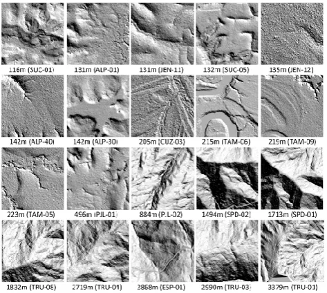
Fig. 1. Shaded relief maps showing the terrain underlying forests along an Andes-to-Amazon elevation gradient of 116 m to 3379 m a.s.l. Site names are shown in parentheses, matching those listed in Table 1. These results are 1.1 m spatial resolution.

1831.5–3379.3 m a.s.l. (Table 2). Hereafter for convenience, we refer to these three groups as lowland, sub-montane and montane landscapes. Among the lowland landscapes, the variance in elevation was very low, with a maximum-recorded standard deviation (SD) of just 6.7 m on the ALP-30 landscape (Fig. 1). Coefficients of variation (CV) in el-evation averaged 1.1 % among lowland landscapes. Slopes on a 5 m×5 m kernel basis ranged from a mean (±SD) of 2.4◦ (2.2◦)to 9.7◦ (5.2◦). Throughout the lowlands, topo-graphic aspect was oriented mostly in the north–south direc-tion (∼154–192◦true N).

Table 1. Description of 25 ha landscapes mapped and analyzed in the Andes-to-Amazon corridor. Soil orders follow the US Department of Agriculture (USDA) soil taxonomy system. Sites labeled with an asterisk (∗) are those considered to be higher in soil fertility, as reported in the literature.

Site Name Center latitude Center longitude MAP (mm) MAT (C) Soil order

Sucusari; SUC-01 −3.2519 −72.9078 2754 26.2 Ultisol

Allpahuayo; ALP-01∗ −3.9491 −73.4346 2760 26.3 Inceptisol

Jenaro Herrera; JEN-11 −4.8781 −73.6295 2700 26.6 Ultisol

Sucusari; SUC-05 −3.2558 −72.8942 2754 26.2 Ultisol

Jenaro Herrera; JEN-12 −4.8990 −73.6276 2700 26.6 Entisol

Allpahuayo; ALP-40 −3.9410 −73.4400 2760 26.3 Entisol

Allpahuayo; ALP-30 −3.9543 −73.4267 2760 26.3 Ultisol

Cuzco Amazonico; CUZ-03∗ −12.5344 −69.0539 2600 24.7 Inceptisol

Tambopata; TAM-06∗ −12.8385 −69.2960 2600 24.0 Inceptisol

Tambopata; TAM-09∗ −12.8309 −69.2843 2600 24.0 Inceptisol

Tambopata; TAM-05 −12.8303 −69.2705 2600 24.0 Ultisol

Paujil; PJL-01 −10.3250 −75.2622 5020 23.1 Ultisol

Paujil; PJL-02 −10.3300 −75.2613 5020 23.1 Ultisol

San Pedro; SPD-02∗ −13.0491 −71.5365 4628 18.5 Inceptisol

San Pedro; SPD-01∗ −13.0475 −71.5423 4341 18.5 Inceptisol

Mirador; TRU-08∗ −13.0702 −71.5559 4341 18.5 Entisol

Trocha Union; TRU-04∗ −13.1055 −71.5893 2678 13.0 Inceptisol

Esperanza; ESP-01∗ −13.1751 −71.5948 1705 12.5 Inceptisol

Trocha Union; TRU-03∗ −13.1097 −71.5995 2678 13.0 Inceptisol

Trocha Union; TRU-01∗ −13.1136 −71.6069 2448 8.0 Inceptisol

3.2 Canopy structure

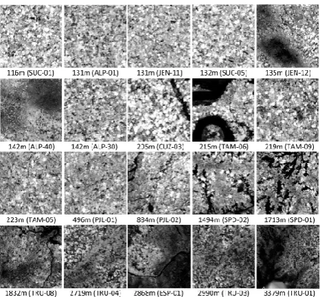
Along the elevation gradient, forest canopy height decreased from a mean (±SD) of 24.5±7.3 m in the lowest lying landscape (SUC-01) to 8.9±5.6 m in the highest landscape (TRU-01) (Fig. 2, Table 2). Note that we masked out the river in TAM-06 in all of our vegetation analyses (Fig. A1). Ele-vation accounted for 72 % of the regional variation in mean canopy height (p< 0.001; RMSE = 2.75 m). This occurred despite the fact that two lowland landscapes on dystrophic white sands (JEN-12, ALP-40) harbored vegetation with lo-cally suppressed canopy height (15.1–16.5 m).

As we crossed the terrain transition from 01 and PJL-02, the canopy opened up with increased prevalence of land-slides at PJL-02 as well as in landscapes SPD-01 and SPD-02 further upslope (Fig. 2). Coefficients of variation in canopy height increased from an average of 33.7 % for all low-land low-landscapes, to 43.4 % for these three sites harboring in-creased landslide activity. At the highest elevations, the land-scapes contained a sparse array of tall (> 25 m) trees embed-ded in a matrix of shorter-statured (3–6 m) vegetation. This resulted in high variance of canopy height while halving of the mean canopy height (Table 2).

We measured all detectable canopy gaps reaching 2 m above ground level in each 25 ha landscape (Fig. 3a). The number of gaps ha−1 increased linearly with elevation (p< 0.05). For example, smaller gaps of < 5 m2 size were 50 % more frequent in the montane than in the lowland land-scapes. This was true for most other gap-size classes as well.

Fig. 2. Vegetation canopy height after removing variation in terrain (see Fig. 1) at 1.1 m spatial resolution throughout forests along the elevation gradient. Site names are shown in parentheses, matching those listed in Table 1.

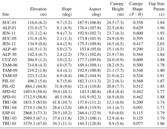
Table 2. Topographic variables for 25 ha Andes-to-Amazon landscapes measured with the CAO lidar. Mean values for ground elevation, slope, aspect, and canopy height are provided with standard deviations in parentheses. The canopy shape ratio is the height of peak canopy volume (P) divided by the 99th percentile total canopy height (H). The canopy gap size parameter (λ)is the negative slope of the power-law relationship between gap size and frequency.

Canopy Canopy Gap Size

Elevation Slope Aspect Height Shape Param

Site (m) (deg) (deg) (m) (P:H) (λ)

SUC-01 116.6 (6.2) 9.7 (5.2) 187.9 (106.8) 24.5 (7.3) 0.558 1.84 ALP-01 131.0 (5.7) 8.1 (6.9) 176.4 (107.8) 22.5 (6.8) 0.629 1.96 JEN-11 131.2 (2.4) 9.4 (7.3) 192.9 (102.7) 23.7 (6.3) 0.600 1.93 SUC-05 131.8 (4.9) 2.1 (1.3) 173.8 (101.9) 24.9 (6.9) 0.595 1.81 JEN-12 134.9 (0.6) 4.6 (2.9) 175.3 (109.8) 16.5 (6.5) 0.417 2.03 ALP-40 141.5 (1.3) 5.0 (3.7) 153.8 (95.0) 15.1 (6.5) 0.290 2.21 ALP-30 142.4 (6.7) 2.4 (2.2) 179.1 (102.6) 21.9 (7.0) 0.564 1.84 CUZ-03 204.9 (1.2) 3.0 (2.2) 177.7 (105.0) 24.0 (9.9) 0.609 1.88 TAM-06 214.8 (4.3) 4.0 (5.7) 169.4 (109.1) 18.2 (9.5) 0.500 1.78 TAM-09 219.2 (1.8) 4.4 (4.1) 192.9 (100.8) 21.1 (7.7) 0.548 1.80 TAM-05 223.3 (2.4) 6.9 (8.4) 186.2 (104.9) 21.0 (6.2) 0.526 1.91 PJL-01 496.2 (5.6) 6.7 (5.6) 182.3 (111.3) 21.2 (6.1) 0.568 1.87 PJL-02 884.1 (64.8) 31.8 (9.6) 121.4 (110.8) 20.8 (7.7) 0.512 1.85 SPD-02 1493.9 (58.6) 39.0 (10.1) 143.5 (80.8) 18.4 (8.4) 0.442 1.77 SPD-01 1712.9 (58.8) 40.1 (9.8) 141.9 (92.3) 16.9 (8.0) 0.462 1.88 TRU-08 1831.5 (83.0) 41.8 (10.7) 137.0 (111.2) 12.1 (6.0) 0.200 1.74 TRU-04 2719.1 (56.5) 28.6 (12.0) 189.8 (119.9) 14.1 (6.7) 0.091 1.73 ESP-01 2868.3 (73.3) 29.5 (10.2) 246.4 (122.9) 9.0 (6.0) 0.115 1.79 TRU-03 2989.5 (67.1) 37.6 (11.8) 129.3 (100.1) 12.9 (6.4) 0.125 1.79 TRU-01 3379.3 (67.0) 34.3 (11.1) 144.3 (120.8) 8.9 (5.6) 0.077 1.86

the lowlands from about 1.75 (larger disturbances) to 2.25 (smaller disturbances) (Fig. 3b). We found a very weak lin-ear decrease inλwith elevation (R2=0.09,p< 0.05).

Using the vertical canopy profile data from the lidar, we discovered systematic changes in canopy architecture with increasing elevation as well as by lowland soil type (Fig. 4). In lowland landscapes, canopies often reached heights of 40–44 m, with the bulk of the canopy volume situated 20– 25 m above ground level (Fig. 4a). We note that the TAM-09 landscape also contained a vegetation layer about 2–3 m above ground, associated with swamp and riparian vegetation found along the Tambopata River. In contrast, the lowland landscapes on the white sands (JEN-12, ALP-40) contained canopies reaching lower maximum heights of 32–37 m, and with leaves more evenly distributed throughout the vertical profile (Fig. 4b).

The canopy P :H shape ratio was inversely correlated with elevation (R2=0.68; P< 0.001; RMSE = 0.11) (Ta-ble 2).P :H was 0.56±0.04 for lowland canopies on non-sand substrates. For non-sands, P :H declined to 0.35±0.08, indicating a groundward shift in the vertical distribution of foliage. Canopies in the four sub-montane sites contained trees that often exceeded 40 m in height, but the vertical partitioning of the foliage shifted groundward in compari-son to the lowland, non-sand landscapes (Fig. 4c). P :H for these sites was 0.50±0.05 (Table 2). We also found a

pronounced understory layer in the 1–5 m height range. Low-statured vegetation cover further increased in the montane landscapes, with nearly all vegetation dominating classes < 10 m in height (Fig. 4d). We note, however, that even the montane forests contained some trees approaching and ex-ceeding 30 m in height.P :H ratios for the montane land-scapes were 0.12±0.05, indicating a strong groundward shift in the vertical partitioning of the vegetation in the high-est Andean Amazon forhigh-ests.

Figure  3  

Fig. 3. (a) Changes in mean canopy gap density with increasing elevation for each 25 ha forest landscape. Gaps are computed to 2 m above ground level (Brokaw, 1985a) in seven gap-size classes from < 5 m2to > 200 m2per gap. (b) Changes in the gap-size frequency scaling coefficientλfor each landscape along the elevation gradient. Symbols are colored by USDA soil order; and dots within circles indicate sites included in elevation-based regression of main text.

observations indicate that gap-colonizing Chusquea bam-boos and ferns dominate in this low-statured montane veg-etation. Regression analyses of these three vertical canopy layers revealed consistent linear increases in the percentage of understory and/or low-statured vegetation cover with ele-vation (Fig. 6).

We also discovered consistent relationships between the number of gaps per hectare and the percentage cover of low-statured vegetation (Fig. 7). Specifically, we found mono-tonic increases in understory cover with increasing gaps ha−1, but at different rates depending upon gap size classes of 0–5 m2to≥200 m2. Steeper regression slopes were com-puted between understory vegetation cover and elevation in the larger gap classes. These patterns were consistent in the 1–3 m, 3–5 m, and 5–10 m understory vegetation height classes. Increases in the number of gaps ha−1in the 0–5 m2 gap-size classes resulted in the slowest increase in understory plant cover. The opposite was true for the largest (≥200 m2) gap class.

Fig. 4. Mean lidar vertical profiles for canopies in (a) lowland, (b) lowland on white sand soils, (c) sub-montane, and (d) montane forest landscapes. Site names match those provided in Table 1.

Figure  6  

3.3 Canopy function

With the VSWIR spectrometer, we mapped canopy spectral characteristics throughout each 25 ha landscape. Sites ESP-01 and TRU-ESP-01 were not imaged due to poor atmospheric conditions during overflight (Fig. 8). Inspection of the color-infrared images, each of which is histogram-matched for comparison, indicated that lowland sites contain a mix of

Fig. 7. Relationships between canopy gap density (see Fig. 3a) and percentage understory canopy cover (see Fig. 6) in seven gap-size classes from < 5 m2to > 200 m2per gap.

canopies with high near-infrared (NIR) reflectance values shown in red, and lower values in blue. The two landscapes containing the highly dystrophic white sand soils (JEN-12, ALP-40) showed larger, semi-contiguous patches of sup-pressed NIR reflectance. Among three of the sub-montane landscapes, the presence of landslides was also obvious as blue linearly shaped patches (Fig. 8). Otherwise, intact canopies in these sub-montane areas showed generally high NIR reflectances. The pattern changed substantially again in the montane landscapes, which showed decreases in NIR re-flectance.

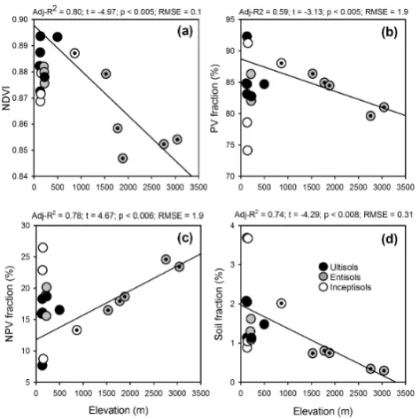
Plotting the VSWIR-derived canopy functional properties against elevation revealed two contrasting patterns (Fig. 9). First, among lowland landscapes, the site-level mean NDVI spanned a range of 0.87 to nearly 0.90 (Fig. 9a). Canopies on Inceptisols (floodplains) in the lowlands had a slightly suppressed average NDVI as compared to canopies on terra

firme Ultisols. Second, the widely varying NDVI in the

Fig. 8. Changes in narrowband, near-infrared reflectance spec-troscopy of forests along the elevation gradient. Images are a combi-nation of near-infrared (800–809 nm), red (650–659 nm), and green (550–559 nm) reflectance. Black areas are image edges, cloud shad-ows (ALP-01), and/or topographic shade (SPD-01/02).

range of PV in the lowlands exceeded the monotonic de-crease among sub-montane to montane sites, spanning nearly 3000 m of elevation gain. Both the lowland and upland PV patterns were mirrored by changes in non-photosynthetic vegetation (NPV) and bare soil fractions (Fig. 9c–d). NPV increased monotonically, while bare soil decreased with ele-vation.

These changes in NDVI, PV, NPV and bare soil fractions occurred despite a lack of elevation trend in the fraction of photosynthetically active radiation intercepted by the vege-tation (fIPAR). In fact, fIPAR remained nearly constant and highly saturated at 0.98 (SD = 0.01) among sites, and there was no relationship with elevation (adj-R2=0.17;p= 0.10).

3.4 Structure–function relationships

We computed Pearson Product Moment correlations to as-sess covariances between the canopy structural and func-tional traits (Table 3). Any relationships described here were significant at thep≤0.05 level. The NDVI was inversely correlated with NPV and bare substrate (S), and positively correlated with canopy height (r=0.83) and shape (P :H; r=0.86). NDVI was consistently negatively correlated with the number of gaps ha−1 in all gap-size classes except for the very largest gaps (r= −0.58 to−0.82), and therefore was also negatively correlated with percentage cover of veg-etation 1–10 m above ground level. Although canopy fIPAR was high and nearly saturated throughout the elevation gradi-ent, it was negatively correlated with the number of canopy

Figure  9  

Fig. 9. Elevation-based changes in (a) NDVI, (b) PV fraction, (c) NPV fraction, and (d) soil fraction derived from imaging spec-troscopy. Data are means for each 25 ha landscape. Symbols are colored by USDA soil order; and dots within circles indicate sites included in elevation-based regression of main text.

gaps ha−1 as well as vegetation cover in the 1–5 m height classes.

Among canopy structural properties, height was positively correlated with shape (P :H) and negatively associated with gaps ha−1_{and low-statured vegetation in all size and height}

classes, respectively (Table 3). The gap-size frequency pa-rameterλwas also negatively correlated with gaps ha−1and vegetation in the 1–3 m height class. Finally, many of the gap-size classes were inter-correlated, while canopy height was not related to the gap size-frequencyλ.

4 Discussion

Table 3. Inter-relationships among landscape-scale canopy functional and structural traits along the elevation gradient. Values are Pearson Product Moment correlation coefficients (r) with bold font indicatingpvalues≤0.05.

% cover in Number of gaps in a size class (m2) per ha height class (m)

NDVI PV NPV S fIPAR Height P:H Gap-sizeλ ≤5 5–10 10–20 20–50 50–100 100–200 ≥200 1–3 3–5 5–10

NDVI – 0.42 −0.58 −0.63 0.66 0.83 0.86 0.18 −0.77 −0.79 −0.74 −0.82 −0.58 −0.73 −0.21 −0.68 −0.82 −0.70

PV – −0.97 0.75 0.21 0.45 0.53 −0.42 −0.06 −0.10 −0.06 −0.09 0.04 −0.10 0.17 −0.13 −0.38 −0.62

NPV – −0.87 0.10 −0.58 −0.66 0.23 0.28 0.31 0.28 0.31 0.17 0.32 −0.05 0.31 0.53 0.67

S – 0.04 0.61 0.63 0.11 −0.55 −0.49 −0.55 −0.48 −0.52 −0.61 −0.29 −0.52 −0.59 −0.57

fIPAR – 0.35 0.38 0.16 −0.64 −0.50 −0.55 −0.54 −0.50 −0.47 −0.47 −0.55 −0.55 −0.48

Height – 0.94 0.04 −0.82 −0.82 −0.71 −0.75 −0.68 −0.63 −0.35 −0.71 −0.87 −0.94

P:H – 0.13 −0.76 −0.85 −0.71 −0.79 −0.65 −0.65 −0.17 −0.66 −0.86 −0.90

Gap-sizeλ – −0.41 −0.52 −0.60 −0.55 −0.53 −0.53 −0.26 −0.48 −0.25 0.16

Gap≤5 m2 – 0.92 0.89 0.87 0.90 0.87 0.68 0.89 0.81 0.63

Gap 5–10 m2 _{– 0.90 0.96 0.80 0.80 0.37 0.86 0.87 0.67}

Gap 10–20 m2 _{– 0.92 0.86 0.86 0.55 0.94 0.86 0.56}

Gap 20–50 m2 – 0.75 0.86 0.37 0.90 0.90 0.62

Gap 50–100 m2 – 0.87 0.76 0.82 0.69 0.48

Gap 100–200 m2 _{– 0.62 0.85 0.75 0.46}

Gap≥200 m2 _{– 0.64 0.38 0.18}

1–3 m cover – 0.90 0.58

3–5 m cover – 0.85

5–10 m cover –

steeper slopes in tectonically active areas, consistent with coarser resolution data for the region (e.g., Regard et al., 2009).

These threshold changes in topography were, to some ex-tent, expressed in non-systematic changes in canopy func-tional traits. For example, we found very wide-ranging val-ues of NDVI, PV, NPV and bare substrate in our 25 ha study landscapes across the lowlands. Wide-ranging lowland vari-ability then gave way to monotonic, and often less exten-sive, changes in these functional metrics above 400 m ele-vation (Fig. 9). Since NDVI, PV and NPV are known cor-relates with canopy greenness, leaf cover, and exposed non-photosynthetic vegetation, respectively (Roberts et al., 1997; Asner et al., 2005; Gamon et al., 1995), our findings highlight the strong degree to which canopy structural and functional variation is linked to regional patterns of geologic, hydro-logic, and soil fertility variation in the lowlands. This find-ing may also reflect reports of widely varyfind-ing community composition, productivity, and carbon storage throughout the western Amazonian lowlands (Quesada et al., 2012; Asner et al., 2012a; Higgins et al., 2012; Aragão et al., 2009; Girardin et al., 2014; Carvalho et al., 2013; Tuomisto et al., 1995).

In contrast to the wide-ranging functional trait variation observed in the lowlands, variability in canopy structural properties was mostly tied to changes in elevation alone. For example, the number of gaps ha−1(Fig. 3) and the per-centage cover of understory vegetation (Fig. 6) were con-sistent in the lowlands and then linearly increased to tree-line. Canopy height and the canopyP :Hratio also declined linearly with elevation (Table 2). Moreover, we discovered systematic changes in the vertical distribution of plant tis-sues in lowland to sub-montane, and to montane forest en-vironments (Fig. 4). Exceptions to these rules were found in the two highly dystrophic, white sand landscapes in northern Peru (JEN-12, ALP-40), which harbored locally suppressed

canopy height and a groundward shift in canopy vertical pro-files. So while elevation is the regionally dominant control on canopy structural characteristics, soil fertility also plays a role in creating structural diversity among a subset of low-land forest types (Fig. 10).

Although we discovered a number of elevation-dependent trends in canopy characteristics, we also found coordi-nated variation among many of the properties. For example, canopy height and shape were highly correlated, and both of these properties were negatively related to gap density (Table 3). Moreover, gap densities increased with elevation (Fig. 3), while canopy height decreased with elevation (Ta-ble 2). In Peruvian forests, canopy height (CH) is highly correlated with aboveground biomass at the stand level (0.4356·CH1.7551; R2=0.89; p< 0.001), whereas stand-level wood density is not (R2=0.08; p=0.16) (Asner et al., 2012c). Therefore, canopy height is a good surrogate for aboveground biomass along our elevation gradient. In Peru, 1 ha field plot studies indicated that aboveground biomass de-creases from about 88–138 Mg C ha−1 _{in the lowlands,}

de-pending upon soil type, to about 47–66 Mg C ha−1_near

tree-line, or up to 66 % overall (Girardin et al., 2014; Huaraca Huasco et al., 2014). After we convert lidar-based estimates of canopy height to aboveground biomass estimates using the Peru equations provided by Asner and Mascaro (2014), we obtain an elevation-dependent trend in aboveground biomass stocks that is within 10 % of the plot-based estimates. Thus our estimated decreases in aboveground biomass at the 25 ha scale corroborate 1 ha plot estimates of biomass decreases with increasing elevation.

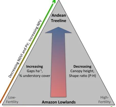
Andean   Treeline  

Amazon  Lowlands   Low-­‐  

FerClity   FerClity  High-­‐   Increasing  

Gaps  ha-­‐1_,   %  understory  cover  

Decreasing  

Canopy  height,     Shape  raCo  (P:H)  

Figure  10  

Decreasing  NDVI  and  PV;    Increasing  NPV,  CH,  P:H  

Fig. 10. Summary of results presented in the study: as elevation increases from the Amazon lowlands to Andean treeline, the for-est canopy undergoes increases in canopy gap density and under-story plant cover, while canopy height and shape ratio (P :H) de-crease. Functional trait metrics of NDVI and fractional PV cover decrease, while fractional NPV cover increases, from low-fertility sites in the lowlands to Andean treeline. A similar trend occurs from low- to high-fertility lowland sites. Additionally, canopy height and the shape ratio increase from low- to high-fertility sites within the lowlands.

among other canopy factors (Hatfield, 1984; Goward and Huemmrich, 1992; Sellers et al., 1995; Myneni et al., 1997). However, we found that fractional intercepted PAR, or fI-PAR, was saturated and nearly constant among the twenty 25 ha landscapes throughout our gradient, so it is unlikely that the NDVI is simply tracking photosynthetically active light absorption. Instead, we found that, as elevation in-creases, the NDVI decreases while gap density increases (Ta-ble 3). We thus hypothesize that the NDVI is suppressed at higher elevations due to slower gap closure rates associated with suppressed NPP.

Although aboveground biomass and NDVI decrease with increasing elevation, we computed a near-constant gap-size scaling parameter λ throughout the elevation gradient (Fig. 3).λis a quantitative index often used to compare and contrast biomass turnover rates in tropical forests (Gloor et al., 2009; Asner et al., 2013; Chambers et al., 2013). Our re-sults thus suggest that turnover rates are relatively constant when ascending from the lowlands into the montane. Not only would this corroborate previous plot-based studies of nearly constant turnover (Girardin et al., 2010), they point out the potential value of airborne remote sensing for gap-size frequency mapping in large forested regions of Amazo-nia. Doing so will improve our understanding of the spatial

distribution of growth and mortality at much broader ecolog-ical scales than can be achieved with field plots.

Our results provide insight into the relationship between gap formation patterns and understory plant cover. Under-story cover increases with elevation (Fig. 10). This trend is driven by increases in gap density, but at differential rates de-pending upon gap size and vegetation height (Fig. 7). It takes about 25–30 times the number of 0–5 m2gaps to produce un-derstory responses created in a single 20–200 m2gap. These results suggest a strong limiting role of low light availabil-ity on understory plant cover in forests spanning the low-land Amazon to the Andean treeline. Although this issue is already well appreciated in the tropical forest literature (Denslow, 1987; Lawton, 1990), quantification of light re-sponse thresholds have remained elusive due to the imprac-ticalities of field measurements in highly heterogeneous un-derstory light environments (Chazdon, 1988). Here we show that, for western Amazonian forests, gaps larger than 5 m2 are associated with the largest understory plant cover values. Independent of gap size or density, the percentage cover of understory plants never exceeds 8 % per hectare for 1–3 m-or 3–5 m-tall plants, while it often reaches but does not ex-ceed 14 % per hectare for plants of 5–10 m in height. These estimates provide the first constraints on models of distur-bance, demography and ecosystem processes in Amazonian forests of widely varying structure and composition.

The Andes-to-Amazon corridor remains virtually unex-plored scientifically. With thousands of valleys, diverse ter-rain conditions, and variable soils, there exists a vast frontier still to be unravelled. Tropical elevation studies have tradi-tionally relied upon field plots that are distributed in sparse patterns on highly variable terrain. Although plot-based stud-ies are key to understanding ecological processes such as productivity and biogeochemical fluxes, field measurements of canopy structural and functional traits are extremely hard to obtain, resulting in limited methods to extend plot-based measurements to larger ecological scales. Using new air-borne remote measurement techniques, we reported a first analysis of landscape-scale canopy functional and structural traits along an Andes-to-Amazon elevation gradient. Inte-grated hyperspectral and lidar measurements allowed us to draw conclusions on the way elevation, terrain and soils af-fect the three-dimensional forest habitat and its dynamics. Our results are a step toward unravelling structural and func-tional composition in one of the most biologically diverse regions of our planet.

Fig. A1. Shade, ground and water mask (black areas) developed from airborne lidar and applied to all imaging spectrometer analyses (see Fig. 8).

Gordon and Betty Moore Foundation, W. M. Keck Foundation, Margaret A. Cargill Foundation, Mary Anne Nyburg Baker and G. Leonard Baker Jr., and William R. Hearst III.

Edited by: K. Thonicke

References

Alves, L. F., Vieira, S. A., Scaranello, M. A., Camargo, P. B., San-tos, F. A. M., Joly, C. A., and Martinelli, L. A.: Forest structure and live aboveground biomass variation along an elevational gra-dient of tropical Atlantic moist forest (Brazil), Forest Ecol. Man-age., 260, 679–691, doi:10.1016/j.foreco.2010.05.023, 2010. Aragão, L. E. O. C., Malhi, Y., Metcalfe, D. B., Silva-Espejo, J. E.,

Jiménez, E., Navarrete, D., Almeida, S., Costa, A. C. L., Salinas, N., Phillips, O. L., Anderson, L. O., Alvarez, E., Baker, T. R., Goncalvez, P. H., Huamán-Ovalle, J., Mamani-Solórzano, M., Meir, P., Monteagudo, A., Patiño, S., Peñuela, M. C., Prieto, A., Quesada, C. A., Rozas-Dávila, A., Rudas, A., Silva Jr., J. A., and Vásquez, R.: Above- and below-ground net primary productiv-ity across ten Amazonian forests on contrasting soils, Biogeo-sciences, 6, 2759–2778, doi:10.5194/bg-6-2759-2009, 2009. Asner, G. P. and Heidebrecht, K. B.: Spectral unmixing of

vegeta-tion, soil and dry carbon cover in arid regions: comparing multi-spectral and hypermulti-spectral observations, Int. J. Remote Sens., 23, 3939–3958, 2002.

Asner, G. P. and Mascaro, J.: Mapping tropical forest carbon: Cal-ibrating plot estimates to a simple LiDAR metric, Remote Sens. Environ., 140, 614–624, 2014.

Asner, G. P., Wessman, C. A., and Archer, S.: Scale dependence of absorption of photosynthetically active radiation in terrestrial ecosystems, Ecol. Appl., 8, 1003–1021, 1998.

Asner, G. P., Elmore, A. J., Hughes, F. R., Warner, A. S., and Vi-tousek , P. M.: Ecosystem structure along bioclimatic gradients in Hawai’i from imaging spectroscopy, Remote Sens. Environ., 96, 497–508, 2005.

Asner, G. P., Knapp, D. E., Kennedy-Bowdoin, T., Jones, M. O., Martin, R. E., Boardman, J., and Field, C. B.: Carnegie Air-borne Observatory: In-flight fusion of hyperspectral imaging and waveform light detection and ranging (LiDAR) for three-dimensional studies of ecosystems, J. Appl. Remote Sens., 1, 013536, doi:10.1117/1111.2794018, 2007.

Asner, G. P., Hughes, R. F., Vitousek, P. M., Knapp, D. E., Kennedy-Bowdoin, T., Boardman, J., Martin, R. E., Eastwood, M., and Green, R. O.: Invasive plants transform the 3-D structure of rain-forests, P. Natl. Acad. Sci., 105, 4519–4523, 2008.

Asner, G. P., Powell, G. V. N., Mascaro, J., Knapp, D. E., Clark, J. K., Jacobson, J., Kennedy-Bowdoin, T., Balaji, A., Paez-Acosta, G., Victoria, E., Secada, L., Valqui, M., and Hughes, R. F.: High-resolution forest carbon stocks and emissions in the Amazon, P. Natl. Acad. Sci., 107, 16738–16742, 2010.

Asner, G. P., Clark, J. K., Mascaro, J., Galindo García, G. A., Chad-wick, K. D., Navarrete Encinales, D. A., Paez-Acosta, G., Cabr-era Montenegro, E., Kennedy-Bowdoin, T., Duque, Á., Balaji, A., von Hildebrand, P., Maatoug, L., Phillips Bernal, J. F., Yepes Quintero, A. P., Knapp, D. E., García Dávila, M. C., Jacobson, J., and Ordóñez, M. F.: High-resolution mapping of forest car-bon stocks in the Colombian Amazon, Biogeosciences, 9, 2683– 2696, doi:10.5194/bg-9-2683-2012, 2012a.

Asner, G. P., Knapp, D. E., Boardman, J., Green, R. O., Kennedy-Bowdoin, T., Eastwood, M., Martin, R. E., Ander-son, C., and Field, C. B.: Carnegie Airborne Observatory-2: Increasing science data dimensionality via high-fidelity multi-sensor fusion, Remote Sens. Environ., 124, 454–465, doi:10.1016/j.rse.2012.06.012, 2012b.

Asner, G. P., Mascaro, J., Muller-Landau, H. C., Vieilledent, G., Vaudry, R., Rasamoelina, M., Hall, J. S., and van Breugel, M.: A universal airborne LiDAR approach for tropical forest carbon mapping, Oecologia, 168, 1147–1160, doi:10.1007/s00442-011-2165-z, 2012c.

Asner, G. P., Kellner, J. R., Kennedy-Bowdoin, T., Knapp, D. E., Anderson, C., and Martin, R. E.: Forest canopy gap distribu-tions in the southern Peruvian Amazon, PLoS ONE, 8, e60875, doi:10.1371/journal.pone.0060875, 2013.

Baker, T. R., Phillips, O. L., Malhi, Y., Almeida, S. A. S., Arroyo, L., Di Fiore, A., Erwin, T., Killeen, T. J., Laurance, S. G., Lau-rance, W. F., Lewis, S. L., Lloyd, J., Manteagudo, A., Neill, D. A., Patino, S., Pitman, N. C. A., Natalino, J., Silva, M., and Mar-tinez, R. V.: Variation in wood density determines spatial patterns in Amazonia forest biomass, Glob. Change Biol., 10, 545–562, 2004.

Brokaw, N. V.: The definition of treefall gap and its effect on mea-sures of forest dynamics, Biotropica, 14, 158–160, 1982. Brokaw, N. V.: Gap-phase regeneration in a tropical forest, Ecology,

66, 682–687, 1985a.

Brokaw, N. V. L.: Treefalls, regrowth, and community structure in tropical forests, in: The ecology of natural disturbance and patch dynamics, edited by: Pickett, S. T. A. and White, P. S., Academic Press, New York, 53–69, 1985b.

of the Southwest Amazon: Detection, Spatial Extent, Life Cy-cle Length and Flowering Waves, PLoS ONE, 8, e54852, doi:10.1371/journal.pone.0054852, 2013.

Chambers, J. Q., Negron-Juarez, R. I., Marra, D. M., Di Vittorio, A., Tews, J., Roberts, D., Ribeiro, G. H. P. M., Trumbore, S. E., and Higuchi, N.: The steady-state mosaic of disturbance and suc-cession across an old-growth Central Amazon forest landscape, P. Natl. Acad. Sci., 110, 3949–3954, 2013.

Chazdon, R. L.: Sunflecks and their importance to forest under-storey plants, Adv. Ecol. Res., 18, 1–63, 1988.

Clauset, A., Shalizi, C. R., and Newman, M. E. J.: Power-law dis-tributions in empirical data, SIAM Review, 51, 661–703, 2007. Colgan, M., Baldeck, C., Féret, J.-B., and Asner, G.: Mapping

Sa-vanna Tree Species at Ecosystem Scales Using Support Vector Machine Classification and BRDF Correction on Airborne Hy-perspectral and LiDAR Data, Remote Sensing, 4, 3462–3480, 2012.

Denslow, J. S.: Tropical rainforest gaps and tree species diversity, Annu. Rev. Ecol. Syst., 18, 431–451, 1987.

Drake, J. B., Dubayah, R. O., Clark, D. B., Knox, R. G., Blair, J. B., Hofton, M. A., Chazdon, R. L., Weishampel, J. F., and Prince, S. D.: Estimation of tropical forest structural characteristics using large-footprint lidar, Remote Sens. Environ., 79, 305–319, 2002. Fine, P. V. A., Mesones, I., and Coley, P. D.: Herbivores promote habitat specialization by trees in Amazonian forests, Science, 305, 663–665, doi:10.1126/science.1098982, 2004.

Fisher, J. I., Hurtt, G. C., Thomas, R. Q., and Chambers, J. Q.: Clus-tered disturbances lead to bias in large-scale estimates based on forest sample plots, Ecol. Lett., 11, 554–563, 2008.

Fyllas, N. M., Patiño, S., Baker, T. R., Bielefeld Nardoto, G., Mar-tinelli, L. A., Quesada, C. A., Paiva, R., Schwarz, M., Horna, V., Mercado, L. M., Santos, A., Arroyo, L., Jiménez, E. M., Luizão, F. J., Neill, D. A., Silva, N., Prieto, A., Rudas, A., Silviera, M., Vieira, I. C. G., Lopez-Gonzalez, G., Malhi, Y., Phillips, O. L., and Lloyd, J.: Basin-wide variations in foliar properties of Ama-zonian forest: phylogeny, soils and climate, Biogeosciences, 6, 2677–2708, doi:10.5194/bg-6-2677-2009, 2009.

Gamon, J. A., Field, C. B., Goulden, M. L., Griffin, K. L., Hartley, A. E., Joel, G., Peñuelas, J., and Valentini, R.: Relationships be-tween NDVI, canopy structure, and photosynthesis in three Cal-ifornian vegetation types, Ecol. Appl., 5, 28–41, 1995.

Gentry, A. H.: Changes in Plant Community Diversity and Floris-tic Composition on Environmental and Geographical Gradients, Ann. Mo. Bot. Gard., 75, 1–34, 1988.

Girardin, C. A. J., Malhi, Y., Aragão, L. E. O. C., Mamani, M., Huaraca Huasco, W., Durand, L., Feeley, K. J., Rapp, J., Silva-Espejo, J. E., Silman, M., Salinas, N., and Whittaker, R. J.: Net primary productivity allocation and cycling of carbon along a tropical forest elevational transect in the Peruvian An-des, Glob. Change Biol., 16, 3176–3192, doi:10.1111/j.1365-2486.2010.02235.x, 2010.

Girardin, C. A. J., Farfan-Rios, W., Garcia, K., Feeley, K. J., Jor-gensen, P. M., Murakami, A. A., Pérez, L. C., Seide, R., Pani-agua, N., Claros, A. F., Maldonado, C., Silman, M., Salinas, N., Reynel, C., Neill, D. A., Serrano, M., Caballero, C. J., Cuadros, M. A. T., Macía, M. J., Killeen, T. J., and Malhi, Y.: Compari-son of biomass and structure in various elevation gradients in the Andes, Plant Ecol. Div., 6, 100–110, 2014.

Gloor, M., Phillips, O. L., Lloyd, J. J., Lewis, S. L., Malhi, Y., Baker, T. R., Lopez-Gonzalez, G., Peacock, J., Almeida, S., de Oliveira, A. C. A., Alvarez, E., Amaral, I., Arroyo, L., Aymard, G., Banki, O., Blanc, L., Bonal, D., Brando, P., Chao, K. J., Chave, J., Davila, N., Erwin, T., Silva, J., Di Fiore, A., Feld-pausch, T. R., Freitas, A., Herrera, R., Higuchi, N., Honorio, E., Jimenez, E., Killeen, T., Laurance, W., Mendoza, C., Mon-teagudo, A., Andrade, A., Neill, D., Nepstad, D., Vargas, P. N., Penuela, M. C., Cruz, A. P., Prieto, A., Pitman, N., Quesada, C., Salomao, R., Silveira, M., Schwarz, M., Stropp, J., Ramirez, F., Ramirez, H., Rudas, A., ter Steege, H., Silva, N., Torres, A., Ter-borgh, J., Vasquez, R., and van der Heijden, G.: Does the dis-turbance hypothesis explain the biomass increase in basin-wide Amazon forest plot data?, Glob. Change Biol., 15, 2418–2430, doi:10.1111/j.1365-2486.2009.01891.x, 2009.

Goward, S. N. and Huemmrich, K. F.: Vegetation canopy PAR ab-sorptance and the normalized difference vegetation index: an assessment using the SAIL model, Remote Sens. Environ., 39, 119–140, 1992.

Hatfield, J. L.: Intercepted photosynthetically active radiation esti-mated by spectral reflectance, Remote Sens. Environ., 14, 65–75, 1984.

Higgins, M. A., Asner, G. P., Perez, E., Elespuru, N., Tuomisto, H., Ruokolainen, K., and Alonso, A.: Use of Landsat and SRTM Data to Detect Broad-Scale Biodiversity Patterns in Northwest-ern Amazonia, Remote Sens., 4, 2401–2418, 2012.

Hodkinson, I. D.: Terrestrial insects along elevation gradients: species and community responses to altitude, Biol. Rev., 80, 489– 513, doi:10.1017/S1464793105006767, 2005.

Huaraca Huasco, W., Girardin, C. A. J., Doughty, C. E., Metcalfe, D. B., Durand, L., Silva-Espejo, J. E., Galiano Cabrera, D., Ara-gao, L. E. O., Rozas Davila, A., Marthews, T. R., Huaraca-Quispe, L. P., Alzamore-Taype, I., Eguiluz-Mora, L., Farfán, W., Cabrera, K. G., Halladay, K., Salinas-Revilla, N., Silman, M., and Malhi, Y.: Seasonal production, allocation and cycling of carbon in two mid-elevation tropical montane forest plots in the Peruvian Andes, Plant Ecol. Div., 7, 125–142, 2014.

Kellner, J. R. and Asner, G. P.: Convergent structural responses of tropical forests to diverse disturbance regimes, Ecol. Lett., 12, 887–897, doi:10.1111/j.1461-0248.2009.01345.x, 2009. Kokaly, R. F., Asner, G. P., Ollinger, S. V., Martin, M. E., and

Wess-man, C. A.: Characterizing canopy biochemistry from imaging spectroscopy and its application to ecosystem studies, Remote Sens. Environ., 113, S78–S91, doi:10.1016/j.rse.2008.10.018, 2009.

Lawton, R. O.: Canopy gaps and light penetration into a wind-exposed tropical lower montane rain forest, Canadian Journal of Forest Research, 20, 659–667, 1990.

Lefsky, M. A., Cohen, W. B., Acker, S. A., Parker, G. G., Spies, T. A., and Harding, D.: Lidar remote sensing of the canopy struc-ture and biophysical properties of Douglas-fir western hemlock forests, Remote Sens. Environ., 70, 339–361, 1999.

Lefsky, M. A., Cohen, W. B., Parker, G. G., and Harding, D. J.: Lidar remote sensing for ecosystem studies, BioScience, 52, 19– 30, 2002.

Malhi, Y., Silman, M., Salinas, N., Bush, M., Meir, P., and Saatchi, S.: Introduction: Elevation gradients in the tropics: laboratories for ecosystem ecology and global change research, Glob. Change Biol., 16, 3171–3175, doi:10.1111/j.1365-2486.2010.02323.x, 2010.

Moser, G., Leuschner, C., Hertel, D., Graefe, S., Soethe, N., and Iost, S.: Elevation effects on the carbon budget of tropical moun-tain forests (S Ecuador): the role of the belowground compart-ment, Glob. Change Biol., 17, 2211–2226, doi:10.1111/j.1365-2486.2010.02367.x, 2011.

Myneni, R. B., Ramakrishna, R. N., and Running, S. W.: Estima-tion of global leaf area index and absorbed PAR using radiative transfer models, IEEE T. Geosci. Remote Sens., 35, 1380–1393, 1997.

Peacock, J., Baker, T. R., Lewis, S. L., Lopez-Gonzalez, G., and Phillips, O. L.: The RAINFOR database: monitoring forest biomass and dynamics, J. Veg. Sci., 18, 535–542, doi:10.1111/j.1654-1103.2007.tb02568.x, 2007.

Quesada, C. A., Phillips, O. L., Schwarz, M., Czimczik, C. I., Baker, T. R., Patiño, S., Fyllas, N. M., Hodnett, M. G., Herrera, R., Almeida, S., Alvarez Dávila, E., Arneth, A., Arroyo, L., Chao, K. J., Dezzeo, N., Erwin, T., di Fiore, A., Higuchi, N., Honorio Coronado, E., Jimenez, E. M., Killeen, T., Lezama, A. T., Lloyd, G., López-González, G., Luizão, F. J., Malhi, Y., Monteagudo, A., Neill, D. A., Núñez Vargas, P., Paiva, R., Peacock, J., Peñuela, M. C., Peña Cruz, A., Pitman, N., Priante Filho, N., Prieto, A., Ramírez, H., Rudas, A., Salomão, R., Santos, A. J. B., Schmer-ler, J., Silva, N., Silveira, M., Vásquez, R., Vieira, I., Terborgh, J., and Lloyd, J.: Basin-wide variations in Amazon forest struc-ture and function are mediated by both soils and climate, Bio-geosciences, 9, 2203–2246, doi:10.5194/bg-9-2203-2012, 2012. Raich, J. W., Russell, A. E., and Vitousek, P. M.: Primary produc-tivity and ecosystem development along an elevational gradient on Mauna Loa, Hawaii, Ecology, 78, 707–722, 1997.

Regard, V., Lagnous, R., Espurt, N., Darrozes, J., Baby, P., Roddaz, M., Calderon, Y., and Hermoza, W.: Geomorphic evidence for recent uplift of the Fitzcarrald Arch (Peru): A response to the Nazca Ridge subduction, Geomorphology, 107, 107–117, 2009. Roberts, D. A., Green, R. O., and Adams, J. B.: Temporal and

spatial patterns in vegetation and atmospheric properties from AVIRIS, Remote Sens. Environ., 62, 223–240, 1997.

Sellers, P. J., Los, S. O., Tucker, C. J., Justice, C. O., Dazlich, D. A., Collatz, G. J., and Randall, D. A.: A global 1◦by 1◦NDVI data set for climate studies. Part 2: The generation of global fields of terrestrial biophysical parameters from the NDVI, Int. J. Remote Sens., 15, 3519–3545, 1995.

Silman, M. R.: Plant species diversity in Amazonian forests, in: Tropical rain forest responses to climate change, edited by: Bush, M. and Flenly, J., Springer-Praxis, London, 2006.

Tanner, E. V. J., Vitousek, P. M., and Cuevas, E.: Experimental in-vestigation of nutrient limitation of forst growth on wet tropical mountains, Ecology, 79, 10–23, 1998.

Terborgh, J.: Maintenance of diversity in tropical forests, Biotrop-ica, 24, 283–292, 1992.

Ticehurst, C., Held, A., and Phinn, S.: Integrating JERS-1 imaging radar and elevation models for mapping tropical vegetation com-munities in Far North Queensland, Australia, Photogramm. Eng. Rem. S., 70, 1259–1266, 2004.

Tuomisto, H., Ruokolainen, K., Kalliola, R., Linna, A., Danjoy, W., and Rodriquez, Z.: Dissecting Amazonian biodiversity, Science, 269, 63–66, 1995.

Ustin, S. L., Roberts, D. A., Gamon, J. A., Asner, G. P., and Green, R. O.: Using imaging spectroscopy to study ecosystem processes and properties, Bioscience, 54, 523–534, 2004.

Vitousek, P. M., Matson, P. A., and Turner, D. R.: Elevational and age gradients in Hawaiian montane rainforest: foliar and soil nu-trients, Oecologia, 77, 565–570, 1988.

Vitousek, P. M., Aplet, G., and Turner, D.: The Mauna Loa environ-mental matrix: foliar and soil nutrients, Oecologia, 89, 372–382, 1992.

Wessman, C. A., Nel, E. M., Bateson, C. A., and Asner, G. P.: A method to access absolute fIPAR of vegetation in spatially complex ecosystems, Proceedings of the Seventh Airborne Earth Science Workshop, NASA Jet Propulsion Laboratory, Pasadena, CA, 409–418, 1998.