R E S E A R C H
Open Access
Numerical methods to simulate moisture
dynamics in fibrous sheet
Hidekazu Yoshioka
*, Kotaro Fukada and Ichiro Kita
*Correspondence:
[email protected] Faculty of Life and Environmental Science, Shimane University, Nishikawatsu-cho 1060, Matsue, Shimane, 690-8504, Japan
Abstract
Comprehension of moisture dynamics in fibrous sheets is indispensable in a wide variety of industrial areas. This paper proposes a practical mathematical model, which is referred to as the 2-D extended porous medium equation (PME), to physically describe moisture dynamics in fibrous sheets under evaporative environment. A numerical method, which is referred to as the 2-D dual-finite volume method (DFVM), to approximate its solutions in a stable manner is also presented so that the moisture dynamics is reasonably simulated. The 2-D DFVM, which can optionally be equipped with isotone numerical fluxes, is examined with test cases to show its satisfactory accuracy and versatility. The parameters and coefficients involved in the mathematical model for a non-woven fibrous sheet are identified with laboratory experiments. Numerical simulation of moisture dynamics in the horizontally or vertically placed sheet is performed as a demonstrative application example of the present model and the numerical method.
Keywords: fibrous sheets; moisture dynamics; extended porous medium equations;
dual finite volume method; non-woven fibrous sheets
1 Introduction
Comprehension of moisture dynamics in fibrous sheets are necessary in a wide variety of industrial areas, such as chemical engineering [, ], environmental engineering [, ], precise agriculture [], and sanitary engineering []. Moisture dynamics in porous media such as fibrous sheets is macroscopic appearance of microscopic liquid water transport in multiply-connected pore network structures [, ]. In practical applications, moisture dy-namics both in fibrous sheets and on their surface, the latter is due to evaporation driven by the humidity dynamics between the sheets and atmosphere [, ], is of importance for manufacturing better products in paper and textile industry [–]. Assessing mois-ture dynamics in non-woven fibrous sheets is therefore indispensable for development of products that are better fit-for-purpose.
Moisture dynamics occurring in the fibrous sheets have been described with nonlinear conservation laws based on the classical fluid dynamics [, ]. Numerically approximat-ing solutions to nonlinear conservation laws requires applications of a conservative and stable numerical method, so that reasonable numerical solutions are obtained, such that positivity and/or monotonicity of certain physical quantities are realized. One common numerical method for nonlinear conservation laws is the finite volume method (FVM)
based on local conservation principles []. The core of the FVM is evaluating numerical fluxes on cell interfaces, which determine accuracy and stability of numerical solutions [, ]. For solving conservation laws with dominant advection in particular, numerical fluxes should guarantee unconditional stability in space and should possess least numer-ical diffusion effects. This issue is more delicate for degenerate conservation laws than for those with non-degenerate counterparts because of possibly vanishing diffusion co-efficients [–]. Mathematically, degeneration of the diffusion coco-efficients significantly affects qualitative behavior of the solutions to the conservation laws [, ]. Degener-ation of diffusion coefficients would cause numerical instabilities even with sufficiently fine meshes when a standard numerical method is utilized []. Handling source terms in nonlinear partial differential equations like conservation laws also requires devised tech-niques for stable computation [, ]. Analyzing the moisture dynamics that we focus on would require sophisticated numerical techniques due to its complexity, which is our motivation of writing this paper with a particular emphasis on numerics.
This paper focuses on an FVM for porous medium equations (PMEs), which govern moisture dynamics in porous media, such as soils [–], fibrous sheets [, , ], and debris materials []. Similar differential equations are encountered in different physical problems, such as heat conduction problems in plasma [, ], combustion of liquids [, ], evaporation dynamics of volatile liquids [], chemotaxis of cells and organisms [, ], and astrophysics []. Detailed, extensive mathematical and numerical analyses on the PMEs have been performed so far [–]. Zambra et al. [] proposed an oscillation-free FVM with the weighted essentially non-oscillatory interpolation. The Discontinuous Galerkin methods are finite volume analogues of finite element methods, which also are conservative [, ]. Finite Volume Element Methods are conservative methods that con-currently use finite element and finite volume discretization schemes, which have also been effectively used for PMEs [, ].
Literature indicate that the concept of the isotonicity on numerical fluxes, originally stated in Ortega and Rheinboldt [] and has later been discussed in Fuhrmann and Lang-mach [], can possibly help develop stable and physically consistent FVMs in a simple manner. According to Fuhrmann and Langmach [], numerical fluxes in the FVMs for nonlinear conservation laws such as PMEs should equip with the isotonicity for computing oscillation-free numerical solutions without extremely fine computational meshes. Their numerical fluxes for the conventional PMEs are isotone and can compute oscillation-free and non-negative numerical solutions; however, they would not be suitable for the PMEs of moisture dynamics in fibrous sheets as later demonstrated in this paper.
discretization method []. Numerical fluxes are evaluated with analytical solutions to linearized local two-point boundary value problems in the DFVM. This numerical tech-nique is referred to as the fitting techtech-nique. Fitting techtech-nique have successfully been used for solving differential equations encountered in a variety of problems, such as option pricing [, ], optimal controls [], and reactive transport phenomena [, ]. Nu-merical fluxes with the fitting technique guarantee first-order spatial convergence for lin-ear problems [, ]. This paper provides an isotone numerical flux specialized for the -D extended PMEs and its application to test cases and a realistic problem. Stability of the present DFVM for the extended PMEs is achieved with a new isotone numerical flux. Nonlinear source terms involved in the extended PMEs are dealt with using an operator-splitting technique [] to compute stable and physically consistent numerical solutions. The rest of this paper is organized as follows. Section presents the -D and -D PMEs. Their regularized counterparts for well-posing the problems are also presented in this section, which are used in numerical computation in this paper. Section presents the discretization procedure of the -D DFVM. Section presents applications of the -D DFVM and -D extended PME to test cases and a realistic problem. Section concludes this paper.
2 Mathematical model
The extended PMEs for moisture dynamics in fibrous sheets subject to evaporation are presented. The -D extended PME [], although it is not explicitly used in this paper, is firstly presented as a reduced counterpart of the present -D model for self-contentedness.
2.1 1-D extended porous medium equation
The -D extended PME was formulated for simulating -D longitudinal moisture dynam-ics occurring in porous media with a striped shape. It is physically reasonable to assume that moisture profiles in such a sheet are transversely homogenous, leading to a longitu-dinally -D model. The saturation at each longitulongitu-dinally -D positionxof a sheet at the timetis denoted byθ=θ(t,x), and is normalized in [, ] as ≤u= (θ–θr)(θs–θr)–≤
whereθsandθrare the maximum (saturated) and minimum (residual) water contents of
the sheet.
Based on the non-dimensionalization method [], the -D extended PME is presented as [, ]
∂u ∂t˜ =
∂ ∂x˜
(m–p)um–p–∂u ∂x˜
+sinα ∂ ∂x˜
um–u–E˜suq ()
subject to appropriate initial and boundary conditions with the non-dimensional variables
˜
t=K
s(m–p)
Dsθs
t, x˜=Ks(m–p) Dsθs
x, and E˜s=
Dsθs
K s(m–p)
Es, ()
whereDs(> ) is the saturated diffusivity,Ks(> ) is the saturated permeability,Es(≥) is
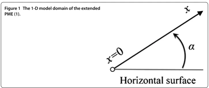
Figure 1 The 1-D model domain of the extended PME (1).
because of the absence of a source term to describe the effect of evaporation. According to the standard theory of evaporation from porous media, it is only as the saturationu that the evaporation rate rapidly decreases to zero []. The pressure headψ(u) and the hydraulic permeabilityK(u) consistent with the -D extended PME () are
ψ(u) =θsDs pKs
–
up
and K(u) =Ksum, ()
respectively. The former reduces to the conventional model whenp→+ [, ]:
ψ(u) =θsDs Ks
lnu. ()
The angleαmay be spatially distributed, but is assumed to be constant in this paper. There exist two contrasting cases on arrangement of the sheets, which are the horizontal (α= ) and vertical cases (α=±.π). The advection term of () vanishes in the horizontal case because of the equalitysinα= . Hereafter, ‘˜·’ representing non-dimensional variables are omitted from the variables for the sake of simplicity of description.
Degenerate advection and diffusion terms of () possibly serve as severe mathematical and computational difficulties at the point of degeneration (u= ) in particular. This paper mitigates the degeneration with a regularization technique [], which modifies () as
∂u ∂t =
∂ ∂x
(m–p)hε(u)
m–p–∂u
∂x
+sinα ∂ ∂x
hε(u)
m–
u–Esuq ()
with the regularization kernel hε(u) = √
u+ε (≥ε) and a small positive constant ε
(= –in this paper), which completely rules out the degeneration. The diffusion
coef-ficient in () is entirely positive over the domain where the PME () is considered. The regularized extended PME () can be written in the flux form as
∂u ∂t +
∂F ∂x = –Esu
q ()
with the fluxF=F(u) given by
F= –(m–p)hε(u)
m–p–∂u
∂x–sinα
hε(u)
m–
Convergence of numerical solutions subject to the regularization to the exact solutions, at least practically, is demonstrated in Section , where utilizing sufficiently small regular-ization parameter does not significantly affects the computational results. This is possibly because the computational errors in the spatial and temporal discretization dominate that due to the regularization. It should be remarked that a similar regularization technique has already been successfully applied to nonlinear advection-diffusion equations with both mathematical and numerical analyzes []. Mathematically rigorous analysis of the regu-larization method for the PMEs, which would be more difficult to perform, is beyond the scope of this paper and will be addressed elsewhere.
2.2 2-D extended porous medium equation
The -D extended PME, which is a -D counterpart of the -D model (), is presented. This model is necessary for simulating essentially -D moisture dynamics in inclined fibrous sheets, such that an application of the -D model is inadequate. The inclination angle is again denoted byα, which is typically horizontal (α= ) or vertical (α=±.π) of the sheet. The -Dx-xCartesian coordinates is taken over the surface of the sheet, which is
identified with a -D flat domainas depicted in Figure . It is assumed for the sake of sim-plicity of description that the sheet is horizontal on thex-direction. Under this
assump-tion, the -D extended PME that governs s the saturationu=u(t,x,x) inis presented as
∂u ∂t =
∂ ∂x
(m–p)um–p–∂u ∂x
+ ∂ ∂x
(m–p)um–p–∂u ∂x
+sinα ∂ ∂x
um–u–Esuq ()
subject to appropriate initial and boundary conditions. The regularized counterpart of () is given following () as
∂u ∂t =
∂ ∂x
(m–p)hε(u)
m–p–∂u
∂x
+ ∂
∂x
(m–p)hε(u)
m–p–∂u
∂x
+sinα ∂ ∂x
hε(u)
m–
u–Esuq ()
to practically mitigate the degeneration. As for the -D model, () can be written in the flux form as
∂u ∂t +
∂F
∂x
+∂F ∂x
= –Esuq ()
with the couple of fluxes (F,F) given by
F
F
=
–(m–p)[hε(u)]m–p–∂∂xu–sinα[hε(u)]m–u
–(m–p)[hε(u)]m–p–∂∂xu
, ()
which is a more suitable expression for application of and FVM.
Finally, in this section, remarks on boundary conditions to be supplemented to the -D extended PME and its regularized counterpart are provided with particular emphasis on the wetting process. From a mathematical viewpoint, at least some boundary conditions should be supplemented to these PMEs in general, since they are partial differential equa-tions of the parabolic-type, although with possible degeneration of the coefficients. From a physical view point, a reasonable boundary condition for simulating a wetting process where a part of the boundary of the domain (∂W) touches liquid water is the Dirichlet
boundary conditionu= meaning that the boundary∂W is fully-wet. Of course, it is
theoretically possible to specify the net flux F·non∂W, but directly measuring the flux
is, at least to our experience, technically not easy. On the other part of the boundary, a simple and appropriate boundary condition is the no-flux condition F·n= where the inner product between the flux vector F and the outward boundary normal vector n van-ishes. This boundary condition represents that no liquid water escapes from the boundary, which is a reasonable assumption for moisture dynamics with evaporation as focused on in this paper later.
3 2-D dual-finite volume method
The discretization procedure of the -D DFVM is explained in this section.
3.1 Spatial discretization
The -D domainis divided into triangular (regular) cells in the usual conforming man-ner. The cells and the nodes are indexed with the natural numbers. The total numbers of the regular cells and nodes are denoted byNeandNn, respectively. Theith node is
de-noted by Pi. The number of nodes directly connected to the node Piis denoted byτ(i)
and thelth of them is denoted by theρ(i,l)th node Pρ(i,l). The length of the edge PiPρ(i,l)is
denoted bydi,l. A dual cell associated with the node Piis denoted bySi, which is defined
as the conventional -D Voronoi cell []
Si=
τ(i)
l=
Si,l=
τ(i)
l=
x|dist(x, Pi) <dist(x, Pρ(i,l))
, ()
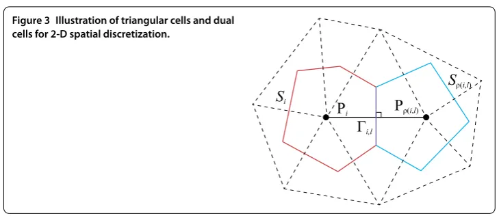
wheredist(·,·) represents the conventional distance function between a couple of points located in the domain. Figure illustrates the -D computational cells used in this paper. The area of the dual cellSiis denoted by|Si|. The length of the outer perimeter of the
sub-cellSi,lof the dual cellSiis denoted byLi,l. The unknownuis attributed to the dual cells
Figure 3 Illustration of triangular cells and dual cells for 2-D spatial discretization.
3.2 Operator-splitting algorithm
The regularized counterpart () is regarded as an advection-diffusion-decay equation hav-ing solution-dependent coefficients, which are discretized fully explicitly at each time step. The -D DFVM thus avoids using nonlinear iteration methods such as the Newton and Pi-card algorithms to realize a simpler and more easily implementable numerical algorithm. An operator-splitting algorithm analogous to that of Li et al. [] specialized for () is in-corporated into the -D DFVM, so that numerical instability due to nonlinearity of the evaporation term is avoided. This approach has successfully been used for conservation laws with nonlinear source terms [, ]. The time increment at each time step is denoted astand the partial differential operators defining the advection and diffusion terms of () asPADand that for the evaporation term asPE: namely,
PADφ=
∂ ∂x
(m–p)hε(φ)
m–p–∂φ
∂x
+ ∂ ∂x
(m–p)hε(φ)
m–p–∂φ
∂x
+sinα ∂ ∂x
hε(φ)
m–
φ and
PEφ= –Esφq
()
for genericφ=φ(x,x). The -D DFVM discretizes () at each time step as
u(k+)=exp(.tPE)exp(tPAD)exp(.tPE)u(k), ()
whereu(k)represents the numerical solution at thekth time step. Although the -D DFVM is unconditionally stable for linear advection-diffusion equations, preliminary computa-tion showed that it is not the case for the extended PMEs iftis too large. The reason of this issue would be the loss of ellipticity of the discretized system as already implied in Pop et al. []. This drawback would be overcome if an implicit treatment of the coefficients is used, which will be addressed in future research. Discretization procedure of the two sub-steps is explained below.
3.3 Evaporation sub-step
At an evaporation sub-step, the equation to be solved at each node is expressed as the ordinary differential equation (ODE)
∂u ∂t = –Esu
LetUibe the nodal value of the numerical solution at the previous time step or that at the
end of the previous advection-diffusion sub-step at theith node. Starting from the formal initial conditionUiat the timet, () witht>tfollows
ui(t) =
⎧ ⎨ ⎩
(max{,φi(Ui,t,t)})
–q ( <q< )
Uiexp(–Es(t–t)) (q= )
()
with
φi(u,t,t) =u–q– ( –q)Es(t–t) ()
foru∈R+. By (), the first evaporation sub-step at thekth time step for theith node is
u∗i =expd(.tPE)u(k) ()
with
expd(.tPE)u(ik)=
⎧ ⎨ ⎩
(max{,φi(ui(k),t+ .t,t)})
–q ( <q< )
u(ik)exp(–Es.t) (q= ),
()
where u∗i represents the updated nodal value, which is used as the initial condition of the advection-diffusion sub-step. The updated nodal value at theith node just after the advection-diffusion sub-step is denoted asu∗∗i . The second evaporation sub-step is then expressed as
u(k+)=expd(.tPE)u∗∗i ()
with
expd(.tPE)u∗∗i =
⎧ ⎨ ⎩
(max{,φi(ui∗∗,t+ .t,t)})
–q ( <q< )
u∗∗i exp(–.Est) (q= ).
()
No restriction onthas to be imposed for each evaporation sub-step because the tem-poral integration on the evaporation term is carried out with the analytical solutions.
3.4 Advection-diffusion sub-step
At the advection-diffusion sub-step, the equation to be solved is given by
∂u ∂t +
∂F
∂x
+∂F ∂x
= . ()
A finite volume discretization is applied to () as explained below.
.. Finite volume formulation
Integrating the () in the dual cellSiwith the application of the Gauss-Green theorem
yields
∂ ∂t
Si uds+
τ(i)
l=
whereFi,lis the numerical flux to be evaluated on the cell face between the dual cellsSi
andSρ(i,l). The first term in the left hand-side of () is evaluated as
∂ ∂t
Si
udx≈ |Si|
dui
dt . ()
The numerical fluxFi,l is evaluated with a fitting technique, which uses the analytical
solutionu˜ of the two-point boundary value problem
∂ ∂s
bρ(i,l)u–aρ(i,l)
∂u ∂s
= ()
along the edge PiPρ(i,l)with the local -D coordinatestaken from Pito Pρ(i,l)and the
bound-ary conditions
u(xi) =ui, u(xρ(i,l)) =uρ(i,l) ()
with
aρ(i,l)= (m–p)
hε(uρ(i,l))
m–p–
and bρ(i,l)= –sinα
hε(uρ(i,l))
m–
n,ρ(i,l), ()
whereuρ(i,l)represents the value ofuon the edge PiPρ(i,l)that is specified later andn,ρ(i,l)
is thex-component of the unit normal vector (n,ρ(i,l),n,ρ(i,l)) having the same direction
with the vector−−−−→PiPρ(i,l). The analytical solutionuis obtained as
u=exp(pi,l)ui–uρ(i,l)
exp(pi,l) –
+ uρ(i,l)–ui
exp(pi,l) –
exp
bρ(i,l)
aρ(i,l)
(s–si)
, ()
which is used for directly evaluating the numerical fluxFi,las
Fi,l=bρ(i,l)u–aρ(i,l)
∂u ∂s
=(m–p)n,ρ(i,l) di,l
hε(uρ(i,l))
m–p–
pi,l
exp(pi,l)ui–uρ(i,l)
exp(pi,l) –
, ()
with the local Peclet number
pi,l= –
n,ρ(i,l)di,lsinα
m–p hε(uρ(i,l))
p. ()
The numerical fluxFi,l is fully specified if the value ofuρ(i,l)is evaluated. A remarkable
point of the -D DFVM is that the Peclet numberpi,lis independent ofuwhenp= : By
(),pi,lwithp= is expressed as
pi,l= –
n,ρ(i,l)di,lsinα
m . ()
.. Numerical flux
The value ofuρ(i,l)is specified to determineFi,l. The three evaluation schemes foruρ(i,l)are
presented in this paper, which are the central (CE) scheme, fully-upwind (FU) scheme, and the isotone (IS) scheme. The CE and FU scheme have been used in Fuhrmann and Langmach [], and the IS scheme is a new numerical method proposed in this paper. The approximationε= is used in this and next sections because it is assumed to be a sufficiently small positive constant such that it does not significantly affect accuracy of numerical solutions.
The CE and FU schemes evaluateuρ(i,l)as
uρ(i,l)=
(ui+uρ(i,l)) ()
and
uρ(i,l)=max(ui,uρ(i,l)), ()
respectively.
The concept of isotonicity is presented in this sub-section for proposing an isotonic numerical flux suited to solving the extended PME. The numerical flux is regarded as a bi-variate function of the non-negative parametersλ,μ≥ as
Fi,l=F˜i,l(λ,μ)|λ=ui,μ=uρ(i,l) ()
with
˜
Fi,l(λ,μ) =
mn,ρ(i,l)pi,l
di,l
uρ(i,l)(λ,μ)
m–exp(pi,l)ui–uρ(i,l)
exp(pi,l) –
. ()
The numerical fluxFi,lis said to be isotone if both
n,ρ(i,l)
∂F˜i,l
∂λ ≥ ()
and
–n,ρ(i,l)
∂F˜i,l
∂μ ≥ ()
for arbitraryλ,μ≥ []. The value ofuρ(i,l)should be determined so that both () and
() are satisfied; however, analytically finding suchuρ(i,l)in generic cases is difficult
be-cause of the nonlinearity ofF˜i,l. An exceptional case is that withp= where the analytical
expression ofuρ(i,l)is found as demonstrated in the next subsection.
.. Isotonicity on the CE scheme
.. Isotonicity on the FU scheme
The FU scheme can potentially mitigate such computational difficulty but has excessive numerical diffusion. In addition, FU scheme with the -D DFVM is not isotone as shown below. The quantitiesn,ρ(i,l)
∂F˜i,l
∂λ and –n,ρ(i,l) ∂F˜i,l
∂μ are calculated forλ≥μ≥ with the FU
scheme as
n,ρ(i,l)
∂F˜i,l
∂λ = ∂ ∂λ
mpi,l
di,l
λm–exp(pi,l)λ–μ
exp(pi,l) –
= m di,l
pi,l
exp(pi,l) –
mexp(pi,l)λ– (m– )μ
λm– ()
and
–n,ρ(i,l)
∂F˜i,l
∂μ = ∂ ∂μ
mpi,l
di,l
λm–μ–exp(pi,l)λ
exp(pi,l) –
= m di,l
pi,l
exp(pi,l) –
λm–
≥, ()
respectively. Similarly, forμ≥λ≥ with the FU scheme, the inequalities are calculated as
n,ρ(i,l)
∂F˜i,l
∂λ = ∂ ∂λ
mpi,l
di,l
μm–exp(pi,l)λ–μ
exp(pi,l) –
= m di,l
pi,lexp(pi,l)
exp(pi,l) –
μm–
≥ ()
and
–n,ρ(i,l)
∂F˜i,l
∂μ = ∂ ∂μ
mpi,l
di,l
μm–μ–exp(pi,l)λ
exp(pi,l) –
= m di,l
pi,l
exp(pi,l) –
mμ– (m– )exp(pi,l)λ
μm–, ()
respectively. By (), () follows if
exp(pi,l) –
m–
m ≥. ()
Similarly, by (), () follows if
exp(–pi,l) –
m–
m ≥. ()
Thus, both () and () are true if
m–
m ≤exp(pi,l)≤ m
demonstrating that the FU scheme is not isotone when the condition () is violated, which is true when the advection is dominant.
.. Isotonicity on the IS scheme
A new evaluation scheme of the numerical flux, the IS scheme, is presented as a possible alternative to the CE and FU schemes. Assumingp= for mathematical tractability, the IS scheme is expressed as
uρ(i,l)=
⎧ ⎨ ⎩
ui (ifexp(pi,l)ui–uρ(i,l)≥)
uρ(i,l) (otherwise).
()
By () and (), isotonicity of the IS scheme follows forexp(pi,l)λ–μ≥ as
n,ρ(i,l)
∂F˜i,l
∂λ = m di,l
pi,l
exp(pi,l) –
λm–mexp(pi,l)λ– (m– )μ
≥ m
di,l
pi,l
exp(pi,l) –
λm–mexp(pi,l)λ– (m– )exp(pi,l)λ
= m di,l
pi,lexp(pi,l)
exp(pi,l) –
λm–
≥ ()
that verifies (). The scheme forexp(pi,l)λ–μ≥ verifies () as
–n,ρ(i,l)
∂F˜i,l
∂μ = m di,l
pi,l
exp(pi,l) –
λm–≥. ()
The proof of the isotonicity of the IS scheme forexp(pi,l)λ–μ< proceeds in an essentially
similar way since
n,ρ(i,l)
∂F˜i,l
∂λ = m di,l
pi,lexp(pi,l)
exp(pi,l) –
μm–≥ ()
and
–n,ρ(i,l)
∂F˜i,l
∂μ = ∂ ∂μ
mpi,l
di,l
μm–μ–exp(pi,l)λ
exp(pi,l) –
=mpi,l di,l
mμ– (m– )exp(pi,l)λ
exp(pi,l) –
μm– > m
di,l
pi,l
exp(pi,l) –
μm–
≥. ()
(), (), and () prove that the IS scheme is isotone. In this paper, for the sake of sim-plicity of analysis, the FU scheme is used for the -D model whenp> . This is because the analytical condition for choosinguρ(i,l)as in () is not available. Nevertheless, for small
.. Temporal integration
Assembling () for every node yields the system of linear ODEs. The -D DFVM finally yields the system of linear ODEs
du
dt =u+ξ, ()
where u = [ui] is theNn-dimensional solution vector,= [i,k] is theNn×Nn-dimensional
matrix arising from the spatial discretization, andξ= [ξi] is theNn-dimensional vector
in-dependent of u. The boundary conditions, if necessary, are included inξ. The system of ODEs () is temporally integrated with theθ-method []. This paper specifiesθ as (Fully implicit scheme). In the -D DFVM, the temporal integration of the advection-diffusion sub step is then expressed as
u∗∗= (I–t)–u∗+ξt, ()
whereIis theNn×Nn-dimensional identity matrix and the vectors u∗∗and u∗are given
by u∗= [u∗i] and u∗∗= [u∗∗i ], respectively. The inversion of the matrixI–is justified be-cause of the positivity conditions of the spatial discretization in the -D DFVM as proved in Yoshioka and Unami []. The linear system is numerically solved with the conventional Gauss-Seidel method whose iteration is terminated until the absolute value of the differ-ence of nodal values between before and after an updating is smaller than –for every
node.
4 Application 4.1 Test cases
The -D DFVM is applied to a series of test cases for its verification of accuracy and stabil-ity. Note that the aim of these test cases is not comparing the -D DFVM with other meth-ods but to confirm its satisfactory convergence to analytical solutions, since the purpose of this paper is establishment of a mathematical model and a simple numerical method that can reasonably simulate the -D moisture dynamics. In each test case, the indepen-dent variables are appropriately scaled without the loss of generality. The -D DFVM is developed in a standard C++ environment. Each unstructured triangular computational mesh in what follows has been generated with free software VORO Ver. . (available at http://www.ocn.ne.jp/~yss/voro.html). The -D DFVM with the operator splitting technique is expected to perform first-order accuracy in time according to Li et al. []. Note that using the Crank-Nicolson scheme (θ = .) in the temporal integration of the advection-diffusion sub-step yields oscillatory numerical solutions in the test cases exam-ined below. The exact solutions in some test cases are partiallyu> , which is physically in-valid. These test cases therefore solely concern computational accuracy of the -D DFVM and do not discuss physical meaning of the solutions.
.. Test:Barenblatt problem
This is a classical, radially symmetric weak solution to the conventional PME that has a sharp and non-smooth profile []. The PME to be solved is given by
∂u ∂t =
∂ ∂x
+ ∂
∂x
whose exact solution, the Barenblatt solution, is expressed fort> as
uBa(t,x,x) =max
,
tm
–(m– )(x
+x)
tm
m–
. ()
A series of structured (square) dual grid with the resolution of ×, ×, ×, and × are examined and the numerical solutions are compared with the exact solution () form= , , and and the convergence rate was estimated for eachm. The time incrementtis set as . throughout this test case. The initial condition is set as u(,x,x) =uBa(.,x,x) to avoid the deltaic singularity of the initial condition at the
timet= ofuBa. The computational domain is set as the square (–, )×(–, ) where
the support of the exact solution does not touch its boundary at least at the timet= . where the exact and numerical solutions are compared. The conventional nodallerror
norm Er between exactuexactand numerical solutionsunumerical, which is defined as
Er=
Nn
Nn
i=
(uexact–unumerical) ()
is used as an error metric throughout this paper. The reason of using structured meshes is to verify exact symmetry of the numerical solutions with respect to thex- andx-axis
that the meshes have. The focus of this test case is on accuracy of the scheme in space rather that in time. The exact and numerical solutions are compared att= ..
Figure (a) through (c) compare the numerical and exact solutions form= , , and with the spatial resolution of ×. Table summarizes the error norms and con-vergence rates. The numerical solutions are certainly axially symmetric but not radially symmetric because of using the structured grid that does not have radial symmetry. The radial symmetricity is recovered and the front position is more accurately captured as the mesh is refined. The computational results show that the order of convergence of the -D DFVM degrades as the parametermfor the nonlinearity increases. The order of con-vergence is almost one for eachm. Qualitatively similar computational results have been obtained form=O().
.. Test:steady problem with evaporation
This second test considers water infiltration from one side (x= ) of a horizontal sheet
(α= andp= ) in evaporative environment []. The domain is set as the unit square (, )×(, ). Assuming thatu= on the boundaryx= , an elementary calculation shows
that the steady solution to this test case is
u(x,x) =max
– (m–q)
Es
m(m+q)x
m–q ,
, ()
which is homogenous in thex-direction. The function in the exact solution is cut to
Figure 4 Comparisons of the numerical and exact solutions for Test 1.The computational results with (a)m= 2,(b)m= 3, and(c)m= 4. The contour lines foru= 0.1nwherenrepresent non-negative integers are depicted: black lines are for numerical solution and grey lines for exact solutions.
Table 1 Computed error norms and the order of convergence for Test 1
Mesh Error norm Order of convergence in space
m = 2 m = 3 m = 4 m = 2 m = 3 m = 4
32×32 3.66E–02 6.29E–02 7.69E–02
64×64 2.12E–02 4.12E–02 5.70E–02 7.88E–01 6.10E–01 4.32E–01
128×128 8.54E–03 2.22E–02 3.40E–02 1.31E+00 8.92E–01 7.45E–01
256×256 3.85E–03 1.25E–02 2.28E–02 1.15E+00 8.29E–01 5.77E–01
increment is set ast= .. Steady numerical solutions are computed starting from the initial guessu= over the computational domain where the homogenous Neumann condition is specified on the boundariesx= ,x= , andx= ; the last one does not
affect computational results since the numerical solutions almost vanish nearx= . The
parametersEs,m, andqcan be chosen such that the support of the exact solution ()
becomes [, .]. The parameterqfor the evaporation term is fixed to ., and examined m= , so thatEs= .. The final time of computation is empirically set ast= at which
Figure 5 Comparisons of the numerical and exact solutions for Test 2.The contour lines for
u= 0.1nwherenrepresent non-negative integers are depicted: black lines are for numerical solution and grey lines for exact solutions.
Table 2 Computed error norms and the order of convergence for Test 2
Time increment
t
Error norm Order of convergence in time
32×16 64×16 128×16 32×16 64×16 128×16
0.01 5.04E–02 5.77E–02 6.05E–02
0.001 6.35E–03 5.01E–03 5.51E–03 9.00E–01 1.06E+00 1.04E+00
0.0001 1.29E–02 5.65E–03 2.31E–03 –3.08E–01 –5.22E–02 3.78E–01
Figure compares the numerical and exact solutions for the spatial and temporal reso-lution of × andt= .. Table summarizes the error norms and convergence rates in time. Table implies that choosing too smalltfor a given computational mesh would not be effective. This is considered due to that the front position of the solution is sensitive to spatial resolution rather than the temporal resolution. This computational re-sult suggests employing fine spatial resolution rather than fine temporal resolution would be effective for analyzing steady problems with the support. The computational result also suggests that both space and time resolution should be fine for computing steady solutions having the source term, which is considered to be due to dependence of the numerical so-lution ontthrough the proposed operator-splitting process.
.. Test:travelling wave solution
The travelling wave solutions available in Nasseri et al. [] are used for examining the present DFVM against the -D extended PME without the source term. A particular em-phasis is put on a comparison of the performances of the FU and IS schemes for evaluation of the numerical fluxes. The equation to be discretized is the extended PME forα= .π without the evaporation term andp= whose exact solution is expressed as
u=
c
+tanh
–m–
mD(x–ct)
–
m–
, ()
Figure 6 Comparisons of the numerical and exact solutions for Test 3.The results with(a)FU scheme and(b)IS scheme. The contour lines foru= 0.05nwherenrepresent non-negative integers are depicted: black lines are for numerical solution and grey lines for exact solutions.
Table 3 Computed error norms and the order of convergence for Test 3
Mesh Error norm Order of convergence in space
FU scheme IS scheme FU scheme IS scheme
348 cells 6.95E–03 5.11E–03
1,296 cells 4.29E–03 3.39E–03 6.98E–01 5.92E–01
4,949 cells 1.67E–03 9.80E–04 1.36E+00 1.79E+00
19,565 cells 7.61E–04 5.96E–04 1.14E+00 7.17E–01
Since the present DFVM reduces to the conventional upwind FVM for small diffusion coefficient, its expected order of accuracy in space is one. The same computational meshes with the previous test cases and the additional, finer mesh with , triangular cells and , dual cells are examined. The numerical and exact solutions are compared at the timet= . The time incrementtis set to be ., which is found to be sufficiently small to for assessing computational accuracy in space of the FU and IS schemes.
Figure (a) and (b) compare the numerical and exact solutions to this test case with the second finest mesh for the -D DFVM with the FU and IS schemes, respectively. Table compares the error norms for the present test case with the FU and IS schemes, showing that the convergence order of the both of the schemes are almost one. It is also shown that the numerical solutions with the IS scheme have several tens present have smaller errors than those with the FU scheme except for the finest mesh. There is no significant quali-tative difference between the obtained numerical solutions with the FU and IS schemes. The results indicate that the IS scheme performs slightly better than the FU scheme for the traveling wave-type solutions.
4.2 Demonstrative application
.. Parameter identification
To be used in applications, the extended PME has three coefficients of the functions ofu to be estimated: the pressure headψ(u), the hydraulic permeabilityK(u), and the evapo-ration rateEsuq. This sub-section presents our experimental results to identify reasonable
ranges of the parameters involved in these coefficients. In the experiments, a non-woven fibrous sheet for water absorption was used where the product number is not presented in this paper. Thickness of the sheet is –(m). The company manufactured this product for
multiple purposes, such as materials for vehicles, materials used in civil engineering, water transportation and adsorption in agricultural fields, and sanitary purposes. The parame-tersθMandθrfor this sheet has been estimated asθM= . andθr= ., respectively.
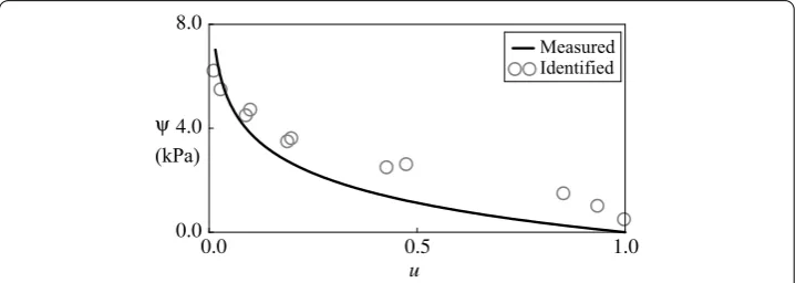
Pressure head As in the case for the conventional hanging water column method to be applied to soil materials [], matric potential was steadily controlled for each fixed pres-sure –n(kPa) with non-negative integers ≤n≤. The moisture weight percentage of the material, which is denoted byw, was measured at each value of the matric potential. This experiment was repeated twice to reduce statistical errors in the identification process of the matric potential. A standard nonlinear least square method is applied to identify the pressure headψ(u).
Figure presents the measured and identifiedψ(u) where the identified parameter val-ues arep= .×–andθsDs
pKs = .×
. The identifiedψ(u) underestimates the
mea-sured counterpart except for smallu, which possibly results in overestimation (underesti-mation) of capillary transport for small (large)u. It would be possible to find more complex but more accurate parameterization ofψ(u) to improve this problem; however, the PMEs with such a coefficient can have higher nonlinearity that is possibly more difficult to nu-merically deal with. This topic is approached in future research and is not focused in this paper. The same applies to the other coefficients.
Hydraulic permeability A tensiometer (Stec Co., Ltd.) was utilized. At the beginning of the experiment, a sheet material that is fully wet was prepared, and it was drained from the wet state until it finalizes the drainage of water. During the drainage process, pres-sure, moisture flux, and moisture weight percentage of the material were measured at one-second interval. This experiment was carried out seven times to reduce statistical er-rors in the identification process of the hydraulic permeability: four times with the pres-sure head of – (cm) and the remaining three with – (cm). The length of the period
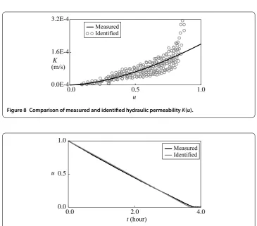
Figure 8 Comparison of measured and identified hydraulic permeabilityK(u).
Figure 9 Comparison of measured and identified variations ofuon the evaporation term.
for the drainage was to (min). Assuming the conventional Darcy’s flux [], the hy-draulic permeability was identified from the experimental results. A standard nonlinear least square method is applied to identify the hydraulic permeabilityK(u) as a function ofu.
Figure presents the measured and identifiedK(u) with the identified parameter values ofKs= .×– (m/s) andm= .. The parameter θpKsDss = .×is thus
identi-fied asDs= .×– (m/s). The measuredK(u) for eachuis subject to fluctuation
because of experimental errors. The identifiedK(u) is found to be an almost median of the measured counterpart for eachu. The identifiedK(u) thus reasonably reproduces the measured counterpart, and both of them qualitatively and qualitatively agree well.
Evaporation rate The evaporation term is identified with a fully wetted sheet placed in a nearly temporally homogenous environment (a closed laboratory room) where the relative of about % to % and the temperature of to degree Celsius. The experimental setting is simple: a fully wetted sheet is placed on an electric balance and its weight is measured at the interval of seconds. The measured data is calibrated with analytical solutions to the ODE ddut = –Esuq. A standard nonlinear least square method is applied to
identify the parametersqandEs.
Figure presents the measured and identified time series ofu. The identified parameter values in the dimensional form areq= .×– andE
s= .×–(/s). Figure
varia-tion ofu. Both the measured and identified time series ofuagrees reasonably well except for smalludespite the present parameterization for the evaporation term is very simple.
.. Computational examples
An application of the presented mathematical model and the numerical method to mois-ture dynamics in the non-woven fibrous sheet is carried out where it is placed horizontally (α= ) or vertically (α= .π). The identified coefficients and parameters in the previous sub-sections are used in the numerical simulation here. The focus here is to track mois-ture dynamics in a sheet with the two contrasting placement patterns under an evaporative environment.
A sheet with a circular shape with the radius of . (m) is considered, which is con-sidered as the domain={(x,x)|x +x< .}in the dimensional form. The finest
computational mesh for the unit circular domain with , triangular cells and , dual cells is used where its spatial scale has been accordingly changed so that the above-mentioned domain is created. The sheet is initially assumed to be dry (u= ), which is specified as the initial condition at the timet= (s). The part of the boundary of the do-main (x,x) with ≤x≤. (m) in the dimensional form is assumed to be fully wet
(u= ) and the other part of the boundary is considered as the no-flux boundary with the conventional zero-flux condition. The time incrementtis set as . in the non-dimensional form, which corresponds to . (s) in the non-dimensional form.
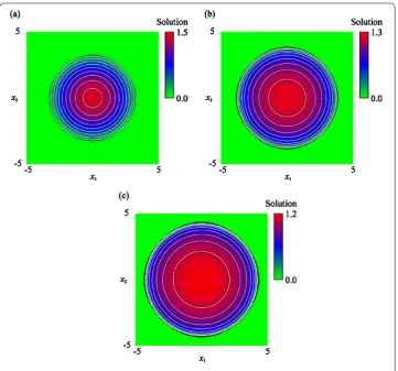
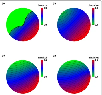
Figure (a) through (d) present the computed saturation at the times .×(s),
.×(s), .×(s), and .×(s) (almost steady state) for the horizontal
displace-ment, respectively. Similarly, Figure (a) through (d) present the computed saturation at the times .× (s), .× (s), .× (s), and .× (s) for the vertical
displacement, respectively. The spatial distributions of the saturationuat the transient states (Figures (a) through (c) and (a) through (c)) are not significantly different between the horizontal and vertical placements; however, they are qualitatively different at the steady state (Figures (d) and (d)). The spatial distribution of the saturationuat the steady state for the horizontal placement is symmetric with respect to the linex+x= ,
but that for the vertical placement is not. This is because the moisture transport is (is not) subject to the gravitational effect for the vertical (horizontal) placement modelled with the nonlinear advection term. Figures (a) and (a) show that the sharp transitions of the solutions are reasonably captured without numerical failure. The obtained computational results show that the numerical solutions obtained do not have unphysical oscillations, overshoots, and undershoots, indicating that the present -D DFVM is able to effectively simulating moisture dynamics subject to the evaporation.
It should be finally noted that both the IS scheme has also been applied to the numerical simulation, but relative error between the numerical solutions with the FU and IS schemes was smaller than several percent. This is considered to be due to the relationshipmpfor the examined non-woven fibrous sheet wherepis sufficiently small to affect the isotonicity of the IS scheme established atp= .
5 Conclusions
Figure 10 Computed saturation at each time for the horizontal displacement.The computational results at(a)0.6×10³(s),(b)1.2×10³(s),(c)4.8×10³(s), and(d)4.8×10⁴(s) (almost steady state), respectively. The contour lines foru= 0.05nwherenrepresent non-negative integers are depicted.
presented in this paper with detailed spatial and temporal integration schemes. The con-cept of isotonicity was effectively incorporated into the evaluation of the numerical flux to compute physically reasonable numerical solutions. An operator-splitting technique based on the analytical solutions to the ODEs was applied to the temporal discretization procedure to handle the problems with nonlinear source terms. Application of the -D DFVM to test cases demonstrated its satisfactory computational accuracy and stability. A demonstrative application example of the -D extended PME and the DFVM showed their potentially high functionality to simulating essentially -D moisture dynamics in fi-brous sheets under evaporative environment.
Figure 11 Computed saturation at each time for the vertical displacement.Computed saturation at the times(a)0.6×10³(s),(b)1.2×10³(s),(c)4.8×10³(s), and(d)4.8×10⁴(s) (almost steady state),
respectively. The contour lines foru= 0.05nwherenrepresent non-negative integers are depicted.
fibrous sheets would involve spatially heterogeneous and/or anisotropic sheets. Hetero-geneity can be partly resolved with the parameters or the coefficients, but appropriate internal boundary conditions will be necessary on the boundary of heterogeneity as in Kuraz et al. [, ]. Transport phenomena of chemical substances whose dynamics typi-cally follows certain conservation laws can be simulated basted on the moisture dynamics with the present model. From a mathematical side, theoretical numerical analysis of the -D DFVM will be performed to deeper comprehend its properties, theoretical order of convergence in particular. Mathematical analysis on the regularization for the nonlinear degenerate parabolic PDEs like PMEs will also be addressed. Approaching from mathe-matical, experimental, and numerical sides to these un-resolved issues will be carried out in future research.
Acknowledgements
The authors thank to the reviewers for providing valuable comments on this paper.
Funding
Japan Society for the Promotion of Science, Research Grant No. 17K15345 partly supports the mathematical analysis part of this research.
Competing interests
Authors’ contributions
HY wrote the paper and performed mathematical and numerical analysis. KF and IK carried out laboratory experiments.
Authors’ information
This paper is a summary of theoretical and experimental analysis carried out by the authors in Shimane University during 2016.
Publisher’s Note
Springer Nature remains neutral with regard to jurisdictional claims in published maps and institutional affiliations.
Received: 17 January 2017 Accepted: 14 July 2017
References
1. Abidin MSBZ, Shibusawa S, Ohaba M, Li Q, Khalid MB. Capillary flow responses in a soil-plant system for modified subsurface precision irrigation. Precis Agric. 2014;15:17-30.
2. Bandyopadhyay A, Ramarao BV, Ramaswamy S. Transient moisture diffusion through paperboard materials. Colloids Surf A, Physicochem Eng Asp. 2002;206:455-67.
3. Bozigian HP, Gendron G, Roberts J. Absorbent hydrogel particles and use thereof in wound dressings. 1999. United States Patent No. 5977428.
4. Lockington DA, Parlange JY, Lenkopane M. Capillary absorption in fibrous sheets and surfaces subject to evaporation. Transp Porous Media. 2008;68:29-36.
5. Ramarao BV. Moisture sorption and transport processes in paper materials. In: Da¸browski A, editor. Studies in surface science and catalysis. Amsterdam: Elsevier; 1999. p. 531-60.
6. Yoshioka H, Kita I, Fukada K. Numerical modelling of nonlinear and degenerate diffusion equations on connected graphs: application to moisture dynamics in non-woven fibrous strip networks. Jpn Soc Industr Appl Math Lett. 2016;8:45-8.
7. Prakotmak P, Soponronnarit S, Prachayawarakorn S. Design of porous banana foam mat to resist moisture migration using a 2-D stochastic pore network and its textural property. Dry Technol. 2014;32(8):981-91.
8. Zheng J, Shi X, Shi J, Chen Z. Pore structure reconstruction and moisture migration in porous media. Fractals. 2014;22(3):1440007.
9. Mikhailov MD, Shishedjiev BK. Temperature and moisture distributions during contact drying of a moist porous sheet. Int J Heat Mass Transf. 1975;18(1):15-24.
10. Cheroto S, Silva Guigon SM, Ribeiro JW, Cotta RM. Lumped-differential formulations for drying in capillary porous media. Dry Technol. 1997;15:811-35.
11. Kumar D, Kumar V, Singh VP. Modeling and dynamic simulation of mixed feed multi-effect evaporators in paper industry. Appl Math Model. 2013;37(1):384-97.
12. Polishchuk A, et al. Cultivation of nannochloropsis for eicosapentaenoic acid production in wastewaters of pulp and paper industry. Bioresour Technol. 2015;193:469-76.
13. Fontana É, et al. Mathematical modeling and numerical simulation of heat and moisture transfer in a porous textile medium. J Text Inst. 2016;107(5):672-82.
14. Landau LD, Lifshitz EM, Pitaevskii LP. Electrodynamics of continuous media. 2nd ed. Oxford: Pergamon Press; 1984. 15. Landau LD, Lifshitz EM. Fluid mechanics. 2nd ed. Oxford: Pergamon Press; 1959.
16. Barth T, Ohlberger M. Finite volume methods: foundation and analysis. Encyclo Comput Mech. 2004. doi:10.1002/0470091355.ecm010.
17. Toro EF. Riemann solvers and numerical methods for fluid dynamics: a practical introduction. 3rd ed. Berlin: Springer; 2009.
18. Toro EF, Garcia-Navarro P. Godunov-type methods for free-surface shallow water flows: a review. J Hydraul Res. 2007;45:736-51.
19. Bessemoulin-Chatard M, Filbet F. A finite volume scheme for nonlinear degenerate parabolic equations. SIAM J Sci Comput. 2012;34:559-83.
20. Kurganov A, Tadmor E. New high-resolution central schemes for nonlinear conservation laws and convection-diffusion equations. J Comput Phys. 2000;160:241-82.
21. Radu FA, Pop IS, Knabner P. Error estimates for a mixed finite element discretization of some degenerate parabolic equations. Numer Math. 2008;109:285-311.
22. Fasano A, Primicerio M. Liquid flow in partially saturated porous media. IMA J Appl Math. 1979;23:503-17. 23. Iaia J, Betelú S. Solutions of the porous medium equation with degenerate interfaces. Eur J Appl Math.
2013;24:315-41.
24. Zhang Q, Wu ZL. Numerical simulation for porous medium equation by local discontinuous Galerkin finite element method. J Sci Comput. 2009;38:127-48.
25. Espedal MS, Karlsen KH. Numerical solution of reservoir flow models based on large time step operator splitting algorithms. In: Fasano A, editor. Filtration in porous media and industrial application. Berlin: Springer; 2000. p. 9-77. 26. Jakobsen ER, Karlsen KH, Risebro NH. On the convergence rate of operator splitting for Hamilton-Jacobi equations
with source terms. SIAM J Numer Anal. 2001;39:499-518.
27. Hayek M. Analytical solution to transient Richards’ equation with realistic water profiles for vertical infiltration and parameter estimation. Water Resour Res. 2016;52:4438-57.
28. Szymkiewicz A, Helmig R. Comparison of conductivity averaging methods for one-dimensional unsaturated flow in layered soils. Adv Water Resour. 2011;34:1012-25.
29. Zha Y, Yang J, Shi L, Song X. Simulating one-dimensional unsaturated flow in heterogeneous soils with water content-based Richards equation. Vadose Zone J. 2013. doi:10.2136/vzj2012.0109.
31. Landeryou M, Eames I, Cottenden A. Infiltration into inclined fibrous sheets. J Fluid Mech. 2005;529:173-93. 32. Pudasaini SP. A novel description of fluid flow in porous and debris materials. Eng Geol. 2016;202:62-73. 33. Bertsch M. Asymptotic behavior of solutions of a nonlinear diffusion equation. SIAM J Appl Math. 1982;42:66-76. 34. Wilhelmsson H. Simultaneous diffusion and reaction processes in plasma dynamics. Phys Rev A. 1988;38:1482-9. 35. Lakkis I, Ghoniem AF. Axisymmetric vortex method for low-Mach number, diffusion-controlled combustion.
J Comput Phys. 2003;184:435-75.
36. Rida SZ. Approximate analytical solutions of generalized linear and nonlinear reaction-diffusion equations in an infinite domain. Phys Lett A. 2010;374:829-35.
37. Okrasiski W, Parra MI, Cuadros F. Modeling evaporation using a nonlinear diffusion equation. J Math Chem. 2001;30:195-202.
38. Borsche R, Gottlich S, Klar A, Schillen P. The scalar Keller-Segel model on networks. Math Models Methods Appl Sci. 2014;24:221-47.
39. Tao Y, Winkler M. Global existence and boundedness in a Keller-Segel-Stokes model with arbitrary porous medium diffusion. Discrete Contin Dyn Syst. 2012;32:1901-14.
40. Haerns V, van Gorder RA. Classical implicit travelling wave solutions for a quasilinear convection-diffusion equation. New Astron. 2012;17:705-10.
41. Antontsev S, Díaz JI, Shmarev S. Energy methods for free boundary problems: applications to non-linear PDEs and fluid mechanics. 1st ed. Boston: Birkhäuser; 2002.
42. Antontsev S, Shemarev S. Evolution PDEs with nonstandard growth conditions: existence, uniqueness, localization, blow-up. 1st ed. Paris: Atlantis Press; 2015.
43. Aronson DG. The focusing problem for the porous medium equation: experiment, simulation and analysis. Nonlinear Anal, Theory Methods Appl. 2016;137:135-47.
44. Zambra CE, Dumbser M, Toro EF, Moraga NO. A novel numerical method of high-order accuracy for flow in unsaturated porous media. Int J Numer Methods Eng. 2012;89:227-40.
45. Yan J. A new nonsymmetric discontinuous Galerkin method for time dependent convection diffusion equations. J Sci Comput. 2013;54:663-83.
46. Albets-Chiko X, Kassions S. A consistent velocity approximation for variable-density flow and transport in porous media. J Hydrol. 2013;507:33-51.
47. Cumming B, Moroney T, Yurner I. A mass-conservative control volume-finite element method for solving Richards’ equation in heterogeneous porous media. BIT Numer Math. 2011;51:845-64.
48. Ortega JM, Rheinboldt WC. Iterative solution of nonlinear equations in several variables. 2nd ed. New York: Academic Press; 1970.
49. Fuhrmann J, Langmach H. Stability and existence of solutions of time-implicit finite volume schemes for viscous nonlinear conservation laws. Appl Numer Math. 2001;37:201-30.
50. Yoshioka H, Triadis D. A regularized finite volume numerical method for the extended porous medium equation relevant to moisture dynamics with evaporation in non-woven fibrous sheets. In: Ohn SY, Chi SD, editors. Model design and simulation analysis. Singapore: Springer; 2016. p. 3-16.
51. Yoshioka H, Unami K. A cell-vertex finite volume scheme for solute transport equations in open channel networks. Probab Eng Mech. 2013;31:30-8.
52. Chernogorova T, Valkov R. Finite volume difference scheme for a degenerate parabolic equation in the zero-coupon bond pricing. Math Comput Model. 2011;54:2659-71.
53. Wang S, Zhang S, Fang Z. A superconvergent fitted finite volume method for Black-Scholes equations governing European and American option valuation. Numer Methods Partial Differ Equ. 2014;31:1190-208.
54. Richardson S, Wang S. Numerical solution of Hamilton-Jacobi-Bellman equations by an exponentially fitted finite volume method. Optimization. 2006;55:121-40.
55. Fiebach A, Glitzky A, Linke A. Uniform global bounds for solutions of an implicit Voronoi finite volume method for reaction-diffusion problems. Numer Math. 2014;128:31-72.
56. Fuhrmann J, Linke A, Langmach H. A numerical method for mass conservative coupling between fluid flow and solute transport. Appl Numer Math. 2011;61:530-53.
57. Roos HG. The ways to generate the Il’in and related schemes. J Comput Appl Math. 1994;53:43-59.
58. Wang S. A novel fitted finite volume method for the Black-Scholes equation governing option pricing. IMA J Numer Anal. 2004;24:699-720.
59. Li Y, Lee G, Jeong D, Kim J. An unconditionally stable hybrid numerical method for solving the Allen-Cahn equation. Comput Math Appl. 2010;60:1591-606.
60. Broadbridge P, White I. Constant rate rainfall infiltration: a versatile nonlinear model: 1. Analytic solution Water Resour Res. 1988;24:145-54.
61. Masoodi R, Pillai KM. Darcy’s law-based model for wicking in paper-like swelling porous media. AIChE J. 2010;56:2257-67.
62. Stewart JM, Broadbridge P. Calculation of humidity during evaporation from soil. Adv Water Resour. 1999;22:495-505. 63. Yoshioka H, Unami K, Fujihara M. A Petrov-Galerkin finite element scheme for 1-D time-independent
Hamilton-Jacobi-Bellman equations. J Jpn Soc Civil Eng Ser A2. 2015;71:I_149-I_160.
64. Mishev ID. Finite volume methods on Voronoi meshes. Numer Methods Partial Differ Equ. 1998;14:193-212. 65. Lee HG, Lee JY. A second order operator splitting method for Allen-Cahn type equations with nonlinear source terms.
Physica A. 2015;432:24-34.
66. Lee HG, Shin J, Lee JY. First and second order operator splitting methods for the phase field crystal equation. J Comput Phys. 2015;299:82-91.
67. Pop IS, Radu F, Knabner P. Mixed finite elements for the Richards’ equation: linearization procedure. J Comput Appl Math. 2004;168:365-73.
68. Knabner P, Angermann L. Numerical methods for elliptic and parabolic partial differential equations. 1st ed. New York: Springer; 2003.
69. Barenblatt GI. On self-similar motions of compressible fluid in a porous medium. Prikl Mat Meh. 1952;16:679-98. 70. Nasseri M, Daneshbod Y, Pirouz MD, Rakhshandehroo GR, Shirzad A. New analytical solution to water content
71. Liu X, Qu C. Long-time behaviour of solutions of a class of nonlinear parabolic equations. Nonlinear Anal, Theory Methods Appl. 2008;69:4470-81.
72. Vázquez JL. The porous medium equation: mathematical theory. Oxford: Oxford University Press; 2007. 73. Jury W, Horton R. Soil physics. 6th ed. Hoboken: Wiley; 2004.
74. Cho CH. On the finite difference approximation for blow-up solutions of the porous medium equation with a source. Appl Numer Math. 2013;65:1-26.
75. Dimova M, Dimova S, Vasileva D. Numerical investigation of a new class of waves in an open nonlinear heat-conducting medium. Cent Eur J Math. 2013;11:1375-91.
76. Guo L, Yang Y. Positivity preserving high-order local discontinuous Galerkin method for parabolic equations with blow-up solutions. J Comput Phys. 2015;289:181-95.
77. Kuraz M, Mayer P, Havlicek V, Pech P. Domain decomposition adaptivity for the Richards equation model. Computing. 2013;95:501-19.