https://doi.org/10.5194/gmd-10-4619-2017 © Author(s) 2017. This work is distributed under the Creative Commons Attribution 4.0 License.
A data model of the Climate and Forecast metadata conventions
(CF-1.6) with a software implementation (cf-python v2.1)
David Hassell1, Jonathan Gregory1,2, Jon Blower3, Bryan N. Lawrence1, and Karl E. Taylor4
1National Centre for Atmospheric Science, Department of Meteorology, University of Reading, Reading, UK 2Met Office Hadley Centre, Exeter, Exeter, UK
3Institute for Environmental Analytics, University of Reading, Reading, UK
4Program for Climate Model Diagnosis and Intercomparison, Lawrence Livermore National Laboratory, Livermore, CA, USA
Correspondence:David Hassell ([email protected]) Received: 29 June 2017 – Discussion started: 10 July 2017
Revised: 31 October 2017 – Accepted: 2 November 2017 – Published: 19 December 2017
Abstract.The CF (Climate and Forecast) metadata conven-tions are designed to promote the creation, processing, and sharing of climate and forecasting data using Network Com-mon Data Form (netCDF) files and libraries. The CF con-ventions provide a description of the physical meaning of data and of their spatial and temporal properties, but they de-pend on the netCDF file encoding which can currently only be fully understood and interpreted by someone familiar with the rules and relationships specified in the conventions docu-mentation. To aid in development of CF-compliant software and to capture with a minimal set of elements all of the inmation contained in the CF conventions, we propose a for-mal data model for CF which is independent of netCDF and describes all possible CF-compliant data. Because such data will often be analysed and visualised using software based on other data models, we compare our CF data model with the ISO 19123 coverage model, the Open Geospatial Consortium CF netCDF standard, and the Unidata Common Data Model. To demonstrate that this CF data model can in fact be imple-mented, we present cf-python, a Python software library that conforms to the model and can manipulate any CF-compliant dataset.
1 Introduction
Network Common Data Form (netCDF) supports a view of data as a collection of self-describing, portable objects that can be accessed through standardised software libraries. For climate scientists, as well as others, it has become a
popu-lar way to create, access, and share array-orientated scientific data (Rew and Davis, 1990; Rew et al., 2006). In this context, “self-describing” means that a file contains, for each data array, an associated description of what it represents scien-tifically, i.e. metadata. NetCDF was developed and is main-tained at Unidata, part of the US University Corporation for Atmospheric Research (UCAR).
The CF (Climate and Forecast) metadata conventions (Eaton et al., 2011, http://cfconventions.org) are a set of rules for storing geoscientific data in netCDF files, with the aims of describing the data, enabling users to identify comparable data held in different files, and facilitating the development of software to extract, process, analyse, and display the data. Initially CF was developed for gridded data from climate and forecast models of the atmosphere and ocean, but its use has subsequently extended to other geosciences, and to observa-tions as well as numerical models. The use of CF is recom-mended where applicable by Unidata.
a previous release of CF would still be compliant with the most recent version.
In general, CF tells data producers how they can provide information they think is important for understanding their data, but it mandates very little metadata. Projects which rec-ommend or require the use of the CF conventions may of course impose additional requirements on data producers, as is done, for instance, by the Coupled Model Intercom-parison Project (https://pcmdi.llnl.gov/mips/cmip5/CMIP5_ output_metadata_requirements.pdf), which in its fifth phase (CMIP5) serves more than 4.2 petabytes of CF-compliant netCDF (CF-netCDF) data.
In this paper, we present a data model which is based on the version of the CF conventions (1.6) which was the latest release at the time of writing. (Since then, 1.7 has been re-leased; see Sect. 7.) By a “data model”, we mean an abstract interpretation of the data, that identifies the elements of the dataset and their scientific intent, and describes how they are related to one another and to the real or model world from which the data were derived. A data model is necessary be-cause it imposes the rules, constraints, and relationships con-necting metadata to the data that are needed to imagine how the quantities included in the dataset should be combined and processed scientifically.
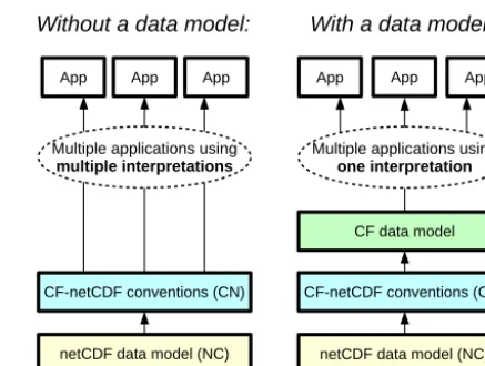
The netCDF interface that underlies CF has an explicit data model (the yellow layer in Fig. 1). CF is defined by the CF-netCDF conventions (the blue layer). The conven-tions have been widely adopted and there are many software applications that work with CF datasets, but up to now a com-prehensive CF data model has not been explicitly proposed (the Open Geospatial Consortium is discussed in Sect. 5.2). Those writing software to process CF-compliant files have implicitly or explicitly adopted data models to serve their own needs, not necessarily considering the whole of the CF convention. Possible CF data models may differ regarding concepts which are more abstract than the storage syntax of netCDF files, and which are therefore not spelled out by the CF convention but become relevant when the data are ma-nipulated or visualised. Divergent interpretations of the data can lead to misunderstandings, inconsistencies, and ineffi-ciencies, and impair the linking of independently developed software tools which might be needed together for the anal-ysis of CF data.
Our aim is to create an explicit data model for CF (the green layer in Fig. 1) to provide an interpretation of the con-ceptual structure of CF which is consistent, comprehensive, and as far as possible independent of the netCDF data model (the yellow layer). We believe that an explicit comprehensive data model will lead to the CF conventions being better un-derstood, will provide guidance during the development of future extensions to the CF conventions, and will help soft-ware developers to design CF-compliant data-processing ap-plications and to build interfaces to other explicit data mod-els.
Without a data model: With a data model:
CF data model
netCDF data model (NC) CF-netCDF conventions (CN)
Multiple applications using
one interpretation
netCDF data model (NC) CF-netCDF conventions (CN)
App
Multiple applications using
multiple interpretations
App App App App App
Figure 1.The benefits of having a CF data model. The CF-netCDF conventions (CN) rely on the netCDF data model (NC) and, at present, a software application is forced to make its own interpreta-tion of the CF-netCDF conveninterpreta-tions – an interpretainterpreta-tion that is likely to be different from that of other applications. The aim of this paper is to propose a comprehensive CF data model that provides a consis-tent interpretation of the conventions, thereby facilitating compati-bility across applications that adopt it. This by no means precludes a variety of software implementations, as there is still considerable flexibility in mapping data model elements onto the data objects needed for a particular application.
1.1 Design criteria for a CF data model
The primary requirement of a data model is that it should be able to describe all existing and conceivable CF-compliant datasets. If we have been successful, then software libraries that adopt our CF data model in constructing their internal data structures will be able to represent and manipulate any CF-compliant dataset.
For our data model, we define a minimal set of elements that are sufficient for accommodating all aspects of the CF conventions. We restrict the elements of a data model to those that are explicitly mentioned in CF, but our data model ments do not have to be irreducible in that a data model ele-ment could describe more than one CF entity. For example, in CF, coordinates and coordinate bounds are distinct enti-ties, but coordinate bounds cannot exist without coordinates. Therefore, it makes sense in our data model to group them into a single element.
Similarly, while it is possible to introduce additional ele-ments not presently needed or used by CF, we believe this would not be desirable because it would increase the likeli-hood of a data model becoming outdated or inconsistent with future versions of CF.
we shall already have set the groundwork for applying CF to other file formats.
1.2 Layout of the paper
In Sect. 3, we introduce the key elements of the CF conven-tions and describe how they are encoded in netCDF files. The relationships between the elements of the CF conven-tions and our proposed CF data model are described in Sect. 4. This data model is compared with other data mod-els in Sect. 5, and a software implementation is presented in Sect. 6. How our CF data model and its software implemen-tation may evolve is discussed in Sect. 7, and a summary and conclusions are given in Sect. 8.
2 The netCDF data model
The existing CF conventions are for use with netCDF files following the netCDF “classic” data model (the yellow layer in Fig. 1). A brief summary of this explicit data model is useful since the CF conventions cannot be described without reference to elements of netCDF.
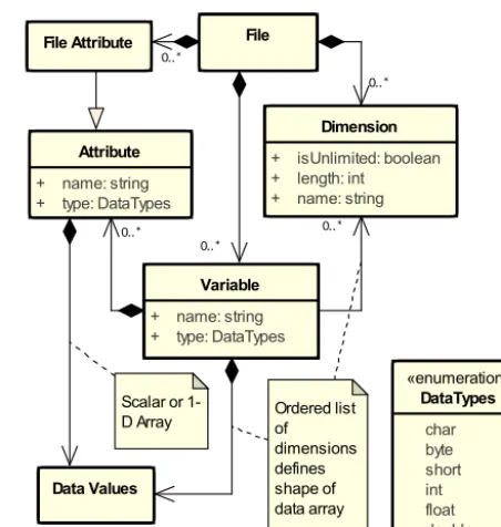
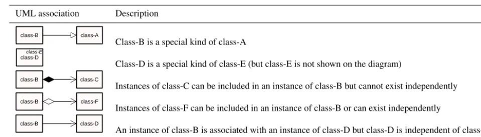
The netCDF classic data model is described using Unified Modeling Language (UML) in Fig. 2. UML provides a stan-dard way to visualise the components of a system and how they relate to each other. In UML, different styles of arrows denote different types of relationship (Table 1). Appendix A provides a primer on the subset of UML used in this paper, and is recommended for readers new to this style of diagram. NetCDF classic files contain data in named variables, which can be single numbers (with no dimensions), one-dimensional arrays (vectors), or multi-one-dimensional arrays, and the dimensions are declared by name in the file. Vari-ables can be of integer, floating point, or character data types. Variables may have attributes, of any data type, at-tached. Attributes can have a single value or consist of a one-dimensional array. NetCDF files also have “global” file attributes which provide information about the dataset as a whole. NetCDF library software has functions to define di-mensions, variables, and attributes, and write and read data.
It is important to appreciate that netCDF itself has no other semantics; for example, while coordinates can be stored in variables and described by attributes, the meanings of these variables and attributes and relationships between them and the variables containing data are not defined by netCDF. NetCDF makes no prescriptions or restrictions regarding the type of metadata which may be stored in the simple data structures that it offers. This flexibility is intended to provide a scope for users and scientific disciplines to develop their own conventions for encoding semantics so that datasets are sufficiently described by those who create them and that they remain valid for those who store and use them. CF is an ex-ample of this.
Variable
+ name: string + type: DataTypes
«enumeration»
DataTypes
char byte short int float double
Dimension
+ isUnlimited: boolean + length: int + name: string
File
Attribute
+ name: string + type: DataTypes
Data Values
Scalar or
1-D Array Ordered listof dimensions defines shape of data array
File Attribute
0..*
0..*
0..* 0..*
0..*
Figure 2.Key components of the netCDF classic data model (corre-sponding to the yellow “NC” layer in Fig. 1) described using UML (Appendix A). Files consist of global attributes, dimensions, and variables. Variables contain attributes and data, and attributes also contain data. Variables, attributes, and dimensions all contain prop-erties, such as a “name” which identifies them in the file. A data array has a data type for all of its elements (e.g. “double” for 64-bit floating point numbers).
The original classic netCDF data model has been “en-hanced” with the addition of several new features, including the ability to organise variables in hierarchical groups. Here, we adopt only one of the new features: we regard the char-acter string as a data type, whereas the classic model treats strings as arrays of individual characters. Logically, these treatments are equivalent, but because strings are easier to manipulate in software codes, it is very likely that they will become a part of CF in the future.
3 The CF conventions
Table 1.The UML class associations used in this paper. See Fig. A1 for a worked example.
UML association Description
class-B class-A
Class-B is a special kind of class-A
class-Dclass-E
Class-D is a special kind of class-E (but class-E is not shown on the diagram)
class-B class-C
Instances of class-C can be included in an instance of class-B but cannot exist independently
class-B class-F
Instances of class-F can be included in an instance of class-B or can exist independently
class-B class-D
An instance of class-B is associated with an instance of class-D but class-D is independent of class-B
In order to reduce storage occupied by netCDF files, the CF conventions provide for lossy packing of data values and non-lossy compression eliminating missing data values. Al-though practically valuable, these mechanisms do not affect our conceptual data model and so we have chosen to describe them in Appendix B rather than in this section.
3.1 Conventions from the netCDF user guide and COARDS
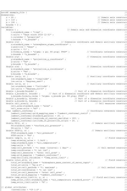
Unidata provides a netCDF user guide (NUG) (Rew et al., 1997), in which they propose some netCDF conventions. CF makes use of these conventions, so we regard them as part of the CF conventions as well (the blue layer in Fig. 1), and they are illustrated in Fig. 3. A one-dimensional variable that has the same name as its dimension (z,x, andyin Fig. 3) is regarded as a coordinate variable. Since CF introduces other types of variables for coordinate data, we sometimes refer to the kind defined in the netCDF user guide as a co-ordinate variable “in the NUG sense”. (By the phrase “co-ordinate variable”, the CF standard document consistently means “coordinate variable in the NUG sense”.) We describe the various kinds of coordinate variables in more detail later (Sect. 3.3). The netCDF user guide proposes a number of conventional attributes; some of these are explicitly included in CF. The guide also contains a statement that it is always allowable to make use of attributes that are not standard-ised by CF. Some of the Unidata attributes recognstandard-ised by CF contain scientific metadata, e.g.source, for the prove-nance of the data, and theunitsof data values (further dis-cussed in Sect. 3.8). Others concern the encoding in netCDF files, e.g.Conventions, stating the netCDF conventions to which the file adheres (line 73 of Fig. 3) and the specifica-tion of a missing data value withmissing_value(line 53 of Fig. 3, indicating that values of−1030correspond to cells for which no data are available, such as ocean points for a quantity measured only over land).
When originally conceived, CF was an extension of the pre-existing COARDS (Cooperative Ocean/Atmosphere Re-search Data Service) netCDF conventions (http://www.ferret.
noaa.gov/noaa_coop/coop_cdf_profile.html). For the sake of backward compatibility of datasets, although CF is now much more comprehensive and flexible than COARDS, CF explicitly upholds some COARDS conventions, which we therefore regard also as part of CF.
3.2 The data and the domain
The overarching purpose of the conventions is to provide conforming datasets with sufficient metadata that they are self-describing, in the sense that each variable in the file has an associated description of what it represents, and that each value can be located (usually in space and time). To meet this objective, we define a data variableV (which might, for example, represent air temperature), over a domaind,
V ≡V (d), (1)
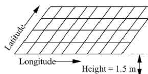
whered represents a set of discrete “locations” in what gen-erally would be a multi-dimensional space, either in the real world or in a model’s simulated world. Thus,V is a function of all its independent dimensions. For example, a variable that is a function of physical location alone would have a three-dimensional discretised domain,
d≡d(z, y, x), (2)
comprising discretised axes of height (z), latitude (y), and longitude (x) (Fig. 4). In CF, the domain may have fewer than three spatial axes, and it may also have any number of non-spatial axes, as in the common case of a variable that is a function time (t). A CF-netCDF file may containNdata vari-ables andMdomains, whereM≤N. Conversely, this means that a given domain may have one or more data variables de-fined at each of its locations. For instance, there could be values for both air temperature and relative humidity at each location in the domaind(z, y, x).
netcdf example_file { // 1
dimensions: // 2
z = 20 ; // Domain axis construct 3 y = 110 ; // Domain axis construct 4 x = 106 ; // Domain axis construct 5 bounds = 2 ; // 6
variables: // 7
double t ; // Domain axis and dimension coordinate construct 8 t:standard_name = "time" ; // 9
t:units = "days since 20161201" ; // 10
t:calendar = "gregorian" ; // 11
t:bounds = "t_bounds" ; // 12
double z(z) ; // Dimension coordinate and domain ancillary construct 13 z:standard_name = "atmosphere_sigma_coordinate" ; // 14
z:positive = "down" ; // 15
z:units = "1" ; // 16
z:formula_terms = "sigma: z ps: PS ptop: PTOP" ; // Coordinate reference construct 17 z:bounds = "z_bounds" ; // 18
double y(y) ; // Dimension coordinate construct 19 y:standard_name = "projection_y_coordinate" ; // 20
y:units = "km" ; // 21
y:bounds = "y_bounds" ; // 22
double x(x) ; // Dimension coordinate construct 23 x:standard_name = "projection_x_coordinate" ; // 24
x:units = "km" ; // 25
x:bounds = "x_bounds" ; // 26
double lon(y, x) ; // Auxiliary coordinate construct 27 lon:standard_name = "longitude" ; // 28
lon:units = "degrees_east" ; // 29
double lat(y, x) ; // Auxiliary coordinate construct 30 lat:standard_name = "latitude" ; // 31
lat:units = "degrees_north" ; // 32
double t_bounds(bounds) ; // Part of a dimension coordinate construct 33 double z_bounds(z, bounds) ; // Part of a dimension coordinate and domain ancillary construct 34 z_bounds:formula_terms = "sigma: z_bounds ps: PS ptop: PTOP" ; // 35
double y_bounds(y, bounds) ; // Part of a dimension coordinate construct 36 double x_bounds(x, bounds) ; // Part of a dimension coordinate construct 37 double cell_area(y, x) ; // Cell measures construct 38 cell_area:standard_name = "area" ; // 39
cell_area:units = "m2" ; // 40
char lambert_conformal ; // Coordinate reference construct 41 lambert_conformal:grid_mapping_name = "lambert_conformal_conic" ; // 42
lambert_conformal:standard_parallel = 25. ; // 43
lambert_conformal:longitude_of_central_meridian = 265. ; // 44
lambert_conformal:latitude_of_projection_origin = 25. ; // 45
double PS(y, x) ; // Domain ancillary construct 46 PS:standard_name = "surface_air_pressure" ; // 47
PS:units = "Pa" ; // 48
double PTOP(y, x) ; // Domain ancillary construct 49 PTOP:standard_name = "air_pressure" ; // 50
PTOP:units = "Pa" ; // 51
double temp(z, y, x) ; // Field construct 52 temp.missing_value = 1.0e30 ; // 53
temp:standard_name = "air_temperature" ; // 54
temp:units = "K" ; // 55
temp:cell_methods = "t: mean (interval: 1 day)" ; // Cell method construct 56 temp:coordinates = "t lat lon" ; // 57
temp:cell_measures = "area: cell_area" ; // 58
temp:grid_mapping = "lambert_conformal" ; // 59
temp:ancillary_variables = "temp_error_limit" ; // 60
double total_wv(y, x) ; // Field construct 61 total_wv:standard_name = "atmosphere_mass_content_of_water_vapor" ; // 62
total_wv:units = "kg m2" ; // 63
total_wv:cell_methods = "t: maximum" ; // Cell method construct 64 total_wv:coordinates = "t lat lon" ; // 65
total_wv:cell_measures = "area: cell_area" ; // 66
total_wv:grid_mapping = "lambert_conformal" ; // 67
double temp_error_limit(z, y, x) ; // Field ancillary construct 68 temp_error_limit:standard_name = "air_temperature standard_error" ; // 69
temp_error_limit:units = "K" ; // 70
// 71
// global attributes: // 72
:Conventions = "CF1.6" ; // 73
:source = "climate model" ; // 74
} // 75
Latitude
Height = 1.5 m Longitude
Figure 4.An example domain defined by three dimensions, one of which is single valued (height).
variables and attributes that are linked to the data variable in various ways defined by the conventions. For instance,temp
is a data variable (line 52 in Fig. 3) with a four-dimensional domain. Itsz,y,x, andt dimensions each have an associ-ated coordinate variable specifying the location at each point along the dimension (thet dimension being implied by the
tscalar coordinate variable; see Sect. 3.3 for details). Note that it is not possible to store a domain in the absence of any data variables (i.e. N≥1), because in the absence of a data variable, CF-netCDF lacks mechanisms to associate the variables from which a domain could be defined. This does not mean that it is disallowed to create a dataset that contains only elements of a domain, but rather that the CF conventions only allow for them to be interpreted collectively as a domain when they are associated with at least one data variable (see Sect. “Interpreting CF-netCDF files” for an example and fur-ther discussion).
Within a CF-netCDF file, dimensions and coordinate vari-ables may be used in the definition of multiple domains, thus reducing redundancy. In our example file,total_wv
is a data variable containing the vertical integral of atmo-spheric water vapour (line 61 in Fig. 3) that has a different domain than thetempdata variable. Itst,y, andx dimen-sions and their coordinates (see Sect. 3.3) are identical to those of temp, so they need not be replicated, but it does not require thezdimension.
3.3 Dimensions and coordinates
NetCDF dimensions establish the size of the index space of data variables, e.g. lines 3–5 in Fig. 3, which specify sizes of 106, 110, and 20 for the x,y, andzdimensions, respec-tively. Each point of the domain of temp is thus defined by a unique set of three indices i=0, . . . , 105, j=0, . . . , 109, and k=0, . . . , 19. NetCDF coordinate variables (in the NUG sense) supply the independent variables on which the data depend. Coordinate variables must be numeric and strictly monotonic, so that each element has a unique value. In our example, we have three coordinate variables, with val-ues z(k),y(j ), andx(i). Each dimension, with its coordi-nate variable if it has one, constitutes an axis of the multi-dimensional space of the domain. The CF conventions quite often use the word “axis” to refer to the physical interpreta-tion of the dimensions of the data.
In many cases, each dimension of a domain can be fully described by a single, strictly monotonic coordinate vari-able (e.g. time, height, latitude, longitude). For more com-plicated cases, however, such as parametric vertical coordi-nates (e.g. dimensionless atmosphere sigma coordicoordi-nates), CF provides a way to record how to compute, from the original dimensional coordinates, dimensional coordinates identify-ing the location of the data in physical space (in the case of sigma, the air pressure). This information is encoded with thestandard_nameandformula_termsattributes of a parametric coordinate variable, e.g. lines 14 and 17 in Fig. 3. Thestandard_nameattribute defines the formula for calculating the dimensional coordinates, which needs to be looked up in the CF conventions document, and the for-mula_terms attribute specifies the values of the formula’s terms. Theatmosphere_sigma_coordinateformula specified in Fig. 3 calculates air pressure from ptop+sigma∗ (ps−ptop), where the values of “ptop” (pressure at the top of the model), “sigma” (the dimensionless coordinates), and “ps” (surface pressure) are taken from the netCDF variables referenced by theformula_termsattribute.
CF also defines “auxiliary coordinate variables” to pro-vide mandatory or optional coordinate information which is additional or alternative to that contained in the coordinate variables in the NUG sense. Auxiliary coordinate variables can be string valued, may contain missing values, and are not necessarily monotonic. For example, we might like to associate the coordinates of a vertical axis with model level number as well as sigma coordinate or to provide location information and station names for the points in a time series (as in Fig. 5). An auxiliary coordinate variable is encoded as a netCDF variable that is referenced by thecoordinates
attribute of a data variable and spans at least one of that data variable’s dimensions, e.g. lines 27, 30, and 57 in Fig. 3. Co-ordinate variables (in the NUG sense) and auxiliary coordi-nate variables (defined by CF) rely on different semantics, and the latter is not a special type of the former, even though they share many characteristics.
refer-11:00 12:00 13:00 14:00 15:00 16:00
Tim
e point
54 38 40 51
Hamburg Princeton
10 −122 −75 −1Livermore Reading name(point,string_max_length)
Long(point) Lat(point)
Figure 5.Auxiliary coordinate variables store “alternative” coordi-nates for dimensions.
enced by the grid_mappingattribute of a data variable, e.g. lines 41 and 59 in Fig. 3.
Some axes have only a single coordinate value. Regret-tably, single-valued coordinates are often omitted from meta-data, although they are very useful; for example, the time information for a field sampled at a single time, for in-stance, 12:15 Z on 14 July 2015, or the level of a single-level field, e.g. air temperature at a height of 1.5 m (Fig. 4). For convenience in storing single-valued coordinates, CF defines a third type of variable containing coordinate data, namely a “scalar coordinate variable”, which requires less netCDF machinery than a dimension of size unity. It is a zero-dimensional netCDF variable that is referenced by the
coordinatesattribute of a data variable, e.g. lines 8 and 57 in Fig. 3.
Calendar time in CF (year, month, day, hour, minute, sec-ond) is encoded with units “time unit since reference date– time” (e.g. line 9 in Fig. 3). The encoded coordinates are the elapsed times since the reference and as such are useful for computing time differences. CF does not use strings for time because they cannot be used for such computations, are in-convenient to standardise, take more storage space, and can-not always be ordered mocan-notonically. The encoding depends on the calendar (e.g. line 10 in Fig. 3), which defines the per-mitted values of the reference date (year, month, and day). The format of the units string conforms to udunits syntax (Sect. 3.8), but the udunits software supports only the real-world Julian/Gregorian calendar and hence is not sufficient for use with CF, which recognises a wide selection of calen-dars, including those for climate models and palaeoclimate. For instance, 31 August 2003 is a valid date in the real-world Gregorian calendar but not in the “360-day” calendar, which has 12 30-day months. In the Gregorian calendar, 12:00 Z on 29 February 2000 is 36 583.5 days since 00:00 Z on 1 Jan-uary 1900, but it is 36 058.5 days in the 360-day calendar.
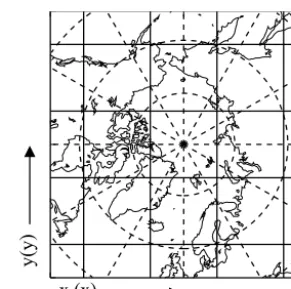
y(y)
x (x)
Figure 6.For grid axes based on a map projection, two-dimensional auxiliary coordinate variables must be used to store longitude and latitude values for each location (latitude–longitude lines dashed; grid lines solid).
3.4 Discrete axes and sampling geometries
A “discrete axis” is one which is not associated with any “continuous” coordinate or auxiliary coordinate variables. A variable is continuous along an axis if it makes physi-cal sense to interpolate along that axis between its values. If that is not the case, then either there are no coordinate values or the coordinate values are discrete indices, whose order may or may not be meaningful. Consider, for exam-ple, an ensemble of model experiments, each of which pro-duces a data variableV (t, z, y, x)containing air pressure as a function of time and spatial location. It may be conve-nient to combine the data variables into a single variable
V (e, t, z, y, x), whereeis the ensemble dimension, defining a discrete axis of ensemble members. The members could be identified by a numeric monotonic coordinate variable with the same name as the dimension containing a member num-ber. Alternatively, it is common for them to be identified by one or more strings, which we could store in auxiliary co-ordinate variables with the ensemble dimension containing, for instance, model names or experiment names. It usually would not make sense to interpolate between ensemble mem-bers, and their order may be immaterial.
have been combined into the one discrete axis. Other exam-ples of DSGs are a vertical profile (variation along a verti-cal axis at a fixed time and spatial location) and a trajectory (variation along a path through space as a function of time). A DSG may also be called a “feature” and the type of DSG is called its “feature type”. The feature type (point, time se-ries, trajectory, profile, etc.) describes the DSG and specifies the dimensionality of the data within the space–time domain. Prior to the introduction of DSGs in version 1.6 of CF, the concept of DSG features was implicit in the sense that they could be inferred from the existence of a discrete axis and well-defined coordinate and auxiliary coordinate variables, but they were not formally described. In general, the netCDF file attributefeatureTypespecifies the DSG feature type for every data variable in the file; but in the cases where the featureType attribute is permitted to be missing, the feature type may be inferred from the dimensions and space–time coordinates alone.
Many DSGs many be stored in one file, but they might have different coordinates, e.g. each time series might have its own set of sampling times (different days or hours of ob-servation), or each profile might have its own set of vertical levels (e.g. air pressure reported by radiosondes). If each fea-ture in a large collection is stored as an individual data vari-able with its own dimensions and coordinate, the file will be cumbersome. If they are combined into a single data variable, a one-dimensional coordinate variable would need to contain the union of all the coordinates (times, levels, etc.) required, and the dimension of the combined data variable might be much larger than needed for the available data, containing a lot of missing data elements.
As an alternative, CF provides three other methods for storing collections of data on DSGs, all intended to allow data with different dimensionality to be stored in a single data variable without wasting so much space. In the “incom-plete multi-dimensional array” representation, the dimension required for the longest feature is used for all features, so that the shorter features must be padded with missing values; this sacrifices storage space to achieve simplicity for reading and writing. The “contiguous ragged array” and “indexed ragged array” representations eliminate the need for padding and thus reduce further the storage required, but they are more complex to pack and unpack. In the former case, each fea-ture in the collection occupies a contiguous block, requiring the size of each feature to be known at the time that it is created. In the latter case, the values of each feature in the collection are interleaved. This representation can therefore be used for real-time data streams that contain reports from many sources, with the data being written as they arrive. The ragged array representations are described in more detail in Appendix B.
Because these storage methods were introduced (in CF version 1.6) at the same time as the recognition and definition of feature types, the two are often thought of as belonging together, but this causes confusion. The featureType is
meta-data, and it refers to the physical construction and interpre-tation of a DSG data variable. The three new storage mecha-nisms for DSGs do not involve any new or distinct physical concepts.
3.5 Bounds and cells
It is often necessary to know the extent of a cell as well as the grid point location, e.g. to calculate the area of a latitude– longitude box or the thickness of a vertical layer. If cell bounds are not provided, then there is no default assumption about cell sizes (an application might reasonably assume that grid points are at the centres of non-overlapping cells, but that is not required by CF).
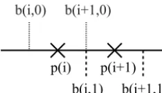
CF provides a way to attach bounds variables to any vari-able containing coordinate data. A bounds varivari-able has an extra dimension to index the vertices of the cells. The sim-plest case is shown for a one-dimensional coordinate vari-able in Fig. 7. In this case, the values p(i) may be a se-ries of successive time instants, for example, midday on 6 and 7 November, bounded by b(i, q)at midnight on 6, 7, and 8 November, withq=0,1. While the bounds for a one-dimensional coordinate variable of dimension(n)could of-ten be stored in a vector of dimension (n+1), CF uses(n,2)
instead as shown because it is convenient for use with the netCDF unlimited dimension, and because it allows cells to be non-contiguous or overlapping. The bounds can be used to test contiguity; in the figure, celliand celli+1 are con-tiguous becauseb(i+1,0)=b(i,1). For multi-dimensional auxiliary coordinate variables, such as the two-dimensional latitude and longitude variables illustrated above, we have to supply the coordinates of each vertex of the polygon and contiguity can similarly be tested by coincidence of vertices. A bounds variable is encoded as a netCDF variable that is referenced by theboundsattribute of a coordinate or aux-iliary coordinate variable and spans the same dimensions (as well as the extra dimension defining the number of vertices), e.g. lines 6, 22, and 36 in Fig. 3.
p(i) p(i+1)
b(i,0) b(i+1,0)
b(i,1) b(i+1,1)
Figure 7.A one-dimensional coordinate variable with grid points p(i)and cell boundariesb(i, q),i=1, . . ., n;q=0,1.
3.6 Variation within cells
CF describes variation within cells by use of “cell meth-ods”. By default, it is assumed that intensive quantities ap-ply at grid points, e.g. temperature values apap-ply at the spa-tial points and instants of time specified by their coordinates, while extensive quantities apply to the entire grid cell, e.g. a precipitation amount (kg m−2) is an accumulation in time. The method may be different for each axis, e.g. precipita-tion amount is intensive in space even though it is exten-sive in time. Because the default is not always obvious, it is recommended that the method be stated explicitly for every axis. Non-default methods include operations such as mean, maximum, minimum, and standard deviation. A zonal-mean variable, for instance, has a cell methods attribute that spec-ifies it is a mean over longitude. A time series of daily max-imum values has cell methods indicating that the values are maxima within their cells in time. The operations recorded by cell methods might affect more than one axis at once, e.g. for the cell methods necessary to describe maximum of the ocean meridional overturning stream function within a depth–latitude cell.
By default, the method for horizontal cells is assumed to have been evaluated over the entire area of the cell. It is, how-ever, possible to limit consideration to only a portion of a cell, e.g. to record that values apply only to the fractions of cells which are land (as opposed to sea).
A further use of cell methods is to characterise climatolog-ical statistics where a series of data points represent sets of subintervals which are not contiguous. There are three kinds to consider:
1. corresponding portions of the annual cycle in a set of years, e.g. decadal averages for January;
2. corresponding portions of a range of days, e.g. the aver-age diurnal cycle in April 1997; and
3. both at once, e.g. the average winter daily minimum temperature from the years 1961 to 1990.
In the latter example, the bounds are 00:00 Z 1 Decem-ber 1961 (beginning of the first day of the first winter) and 00:00 Z 1 March 1991 (end of the last day of the last win-ter), and the cell methods indicate the values are a minimum within days, a mean over a season, and a mean over years.
Cell methods are encoded in the cell_methods at-tribute of a data variable, e.g. line 56 in Fig. 3. In this ex-ample, the cell methodt: mean (interval: 1 day)
specifies that data values are means over the time dimension (i.e. temporal averages) calculated from daily samples. Note that this netCDF file does not contain a dimension for time, but it is sufficient that one is implied by the time scalar coor-dinate variable on line 8.
3.7 Ancillary data
When metadata to describe the data depend on location within the domain, they are stored in independent variables called ancillary data variables. For example, each value of an array of instrument data may have associated measures of uncertainty or of the status of the recording instrument. An ancillary data variable is encoded as a netCDF variable that is referenced by theancillary_variablesattribute of a data variable and spans a subset of the data variable’s di-mensions, e.g. lines 60 and 68 in Fig. 3.
3.8 Units and standard name
A range of attributes is available, introduced by the netCDF user guide or CF, providing metadata for interpreting the val-ues of individual variables or about the dataset as a whole. In this section, we discuss the two most important of these.
CF requires all variables with values (data variables, co-ordinate variables, etc.) to have units unless they contain di-mensionless numbers or cell boundary values. The units are specified by a string attribute (e.g. lines 9 and 55 of Fig. 3), formatted according to the Unidata udunits conventions (Em-merson, 2007), which support many possible units and vari-eties of syntax, e.g. metre, meter, meters, m, km, cm, second, s, kelvin, K, Pa, W m-2, W/m∧2, kg/m2/s, 1 (or any number). Many non-SI units are also supported by udunits, e.g. de-gree, degree_north, degree_N, percent (equivalent to 0.01), ppm (equivalent to 1e-6), mbar, mile, degC, degF, hours, and days.
For systematic identification of the physical quantity con-tained in variables, CF defines a “standard name” string at-tribute (e.g. lines 28, 54 and 62 of Fig. 3), with permissible values listed in the standard name table (http://cfconventions. org/standard-names.html), which includes precise defini-tions. The standard name table is managed by a community process and is continually expanding – version 44 of the ta-ble, released in May 2017, contains 2847 standard names.
Scalar Coordinate
Variable
Data Variable
Boundary Variable NC::Variable
Auxillary Coordinate
Variable
Grid Mapping Variable «abstract»
Generic Coordinate
Variable Coordinate
Variable
Cell Measure Variable
Ancillary Data Variable NC::Dimension
Dimension
NC::Attribute Formula Terms
Cell Methods
0..1 1..*
0..* 0..*
0..*
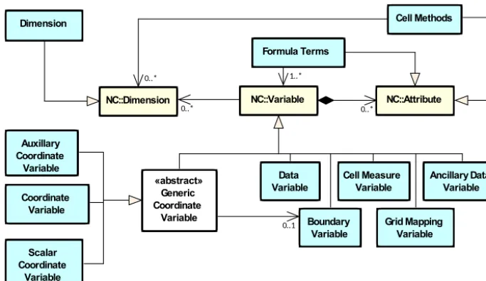
Figure 8.The relationships between CF-netCDF elements (corresponding to the blue CN layer in Fig. 1) and their corresponding netCDF variables, dimensions, and attributes (the yellow NC layer in Fig. 1) described using UML (Appendix A). It is useful to define an abstract generic coordinate variable that can be used to refer to coordinates when the their type (coordinate, auxiliary, or scalar coordinate variable) is not an issue. The CF convention details the mechanisms which are used in the netCDF file to express the relationships among the CF-netCDF elements, but these are not shown in the UML.
sea water potential temperature. Standard names are often longer than the terms familiarly used by the experts in par-ticular discipline, because they answer the question, “What does this mean?”, rather than the question, “What do you call this?”. For example, the quantity often called “precip-itable water” by meteorologists has the standard name of atmosphere_mass_content_of_water_vapor. Standard names have a detailed description which further defines parts of the name; for example, the description of the standard name land_ice_calving_rate notes that “land ice” means glaciers, ice caps, and ice sheets resting on bedrock, and the land ice calving rate is the rate at which ice is lost per unit area through calving into the ocean. Each standard name also implies particular physical dimensions (mass, length, time, and other dimensions corresponding to SI base units, ex-pressed as a “canonical unit”); for example, large-scale rain-fall amount (canonical unit kg m−2), large-scale rainfall flux (kg m−2s−1), and large-scale rainfall rate (m s−1) are all dif-ferent in CF, although they might all be vaguely referred to as “large-scale rain”.
Standard names have been defined for both more general and more specific quantities, for different applications, e.g. ocean_mixed_layer_thickness and ocean_mixed_layer_thickness_defined_by_temperature. Some standard names require the existence of ad-ditional metadata and/or constraints on the val-ues of the variables with which they are associ-ated. For example, the standard name of down-welling_radiance_per_unit_wavelength_in_air requires there to be a coordinate variable storing the radiation wavelength.
The CF conventions use size one or scalar coordinate vari-ables (Sect. 3.3) and the cell_methods attribute (Sect. 3.6) to describe some aspects of a variable, and this means standard names do not always correspond to identities of variables in other file formats. For instance, to describe the time-mean air temperature at 1.5 m above the ground, air_temperature alone is the standard name; “time-mean” is described by cell_methods and the height as a coordinate.
4 A CF data model
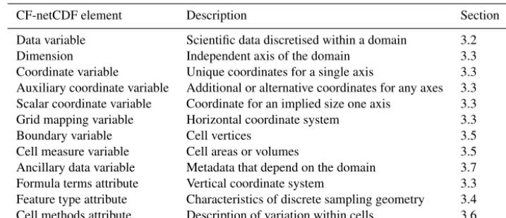
Table 2.The elements of the CF-netCDF conventions, a brief description of each, and the section in which it is described in more detail. The relationships to netCDF entities are shown in Fig. 8.
CF-netCDF element Description Section
Data variable Scientific data discretised within a domain 3.2
Dimension Independent axis of the domain 3.3
Coordinate variable Unique coordinates for a single axis 3.3
Auxiliary coordinate variable Additional or alternative coordinates for any axes 3.3 Scalar coordinate variable Coordinate for an implied size one axis 3.3
Grid mapping variable Horizontal coordinate system 3.3
Boundary variable Cell vertices 3.5
Cell measure variable Cell areas or volumes 3.5
Ancillary data variable Metadata that depend on the domain 3.7
Formula terms attribute Vertical coordinate system 3.3
Feature type attribute Characteristics of discrete sampling geometry 3.4 Cell methods attribute Description of variation within cells 3.6
CF-netCDF elements to the components of netCDF files. To clarify these connections, the example netCDF file shown in Fig. 3 indicates how its elements relate to the constructs of our CF data model.
4.1 The field construct
The field construct is central to our CF data model and in-cludes all the other constructs (Fig. 9). A field corresponds to a CF-netCDF data variable with all of its metadata. All CF-netCDF elements are mapped to some element of the CF field construct, as we describe in following subsections, and the field constructs completely contain all the data and meta-data which can be extracted from the file using the CF ventions. Note that the constructs contained by the field con-struct cannot exist independently, as is indicated by the na-ture of the class associations shown in Fig. 9 (see Table 1 for details).
The field construct consists of a data array and the defi-nition of its domain (i.e.V (d)in Eq. 1), ancillary metadata fields defined over the same domain, and cell method con-structs to describe how the cell values represent the varia-tion of the physical quantity within the cells of the domain (Fig. 9). Because the CF conventions do not mention the con-cept of the domain, we do not regard it as a construct of the data model. Instead, the domain is defined collectively by various other constructs included in the field. All of the data model constructs are listed in Table 3, which refers to the sections and figures in which they are fully described. All of the constructs contained by the field construct are optional (as indicated by “0..*” in Fig. 9). The only component of the field which is mandatory is the data array.
The field construct also has optional properties to de-scribe aspects of the data that are independent of the domain. These correspond to some netCDF attributes of variables (e.g. the units, long_name, and standard_name; Sect. 3.8), and some netCDF global file attributes (e.g. “history” and
“institution”). We use the term “property”, rather than “at-tribute”, because not all CF-netCDF attributes are proper-ties in this sense – some CF-netCDF attributes are used to point to (i.e. reference) other netCDF variables and so only describe the data indirectly (e.g. the “coordinates” attribute; Sect. 3.3), and others have structural functions in the CF-netCDF file (e.g. the “Conventions” attribute). In the data model, we consider that netCDF global file attributes apply to every data variable in the file, except where they are su-perseded by netCDF data variable attributes with the same name. This interpretation of global file attributes is not stated in the CF conventions, but for our data model it is necessary because there is no notion of a file. Hence, metadata stored in attributes of the file as a whole have to be transferred to the field construct. If present, the global file attribute featureType applies to every data variable in the file with a discrete sam-pling geometry (Sect. 3.4). Hence, we regard feature type as a property of the field construct.
The standard_name property (Sect. 3.8) constrains the units property (i.e. only certain units are consistent with each standard name) and in some cases also the dimensions that a data variable must have. These constraints, however, do not supply any further information – they are just for self-consistency. This is also the case for the feature type prop-erty, which imposes some requirements on the axes the do-main must have. Following our aim of constructing a mini-mal data model, we do not regard the standard name nor fea-ture type as separate constructs within the field, because they do not depend on any other construct for their interpretation. This is unlike a cell method, for instance, which depends on the data variable’s dimensions for its interpretation.
4.2 Domain axis construct and the data array
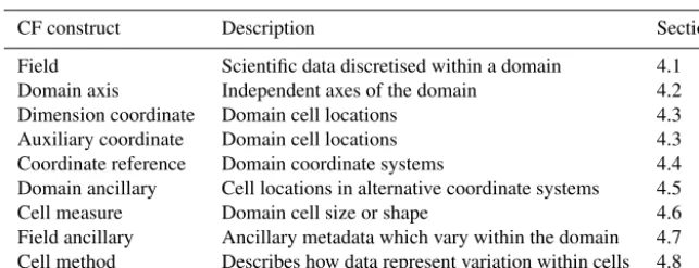
CF-Table 3.The constructs of our CF data model, a brief description of each, and the section in which it is described in more detail. The relationships between the constructs and CF-netCDF elements are shown in Figs. 9–11.
CF construct Description Section
Field Scientific data discretised within a domain 4.1
Domain axis Independent axes of the domain 4.2
Dimension coordinate Domain cell locations 4.3
Auxiliary coordinate Domain cell locations 4.3
Coordinate reference Domain coordinate systems 4.4
Domain ancillary Cell locations in alternative coordinate systems 4.5
Cell measure Domain cell size or shape 4.6
Field ancillary Ancillary metadata which vary within the domain 4.7 Cell method Describes how data represent variation within cells 4.8
netCDF, it is usually defined either by a netCDF dimension or by a scalar coordinate variable, which implies a domain axis of size one (Sect. 3.3). The field construct’s data array spans the domain axis constructs of the domain, with the optional exception of size one axes, because their presence makes no difference to the order of the elements. Hence, the data array may be zero-dimensional (i.e. scalar) if there are no domain axis constructs of size greater than one.
When a collection of DSG features has been combined in a data variable using the incomplete orthogonal or ragged rep-resentations to save space, the axis size has to be inferred, but we regard this as an aspect of unpacking the data, rather than its conceptual description. In practice, the unpacked data ar-ray may be dominated by missing values (as could occur, for example, if all features in a collection of time series had no common time coordinates), in which case it may be prefer-able to view the collection as if each DSG feature were a separate variable (Sect. 3.4), each one corresponding to a dif-ferent field construct.
4.3 Coordinates: dimension coordinate and auxiliary constructs
Coordinate constructs (Fig. 10) provide information which locate the cells of the domain and which depend on a sub-set of the domain axis constructs. As previously discussed, there are two distinct types of coordinate construct: a dimen-sion coordinate construct provides monotonic numeric coor-dinates for a single domain axis, and an auxiliary coordinate construct provides any type of coordinate information for one or more of the domain axes.
In both cases, the coordinate construct consists of a data array of the coordinate values which spans a subset of the do-main axis constructs, an optional array of cell bounds record-ing the extents of each cell, and properties to describe the coordinates (in the same sense as for the field construct). An array of cell bounds spans the same domain axes as its coor-dinate array, with the addition of an extra dimension whose size is that of the number of vertices of each cell. This extra dimension does not correspond to a domain axis construct
since it does not relate to an independent axis of the domain (for example, the boundsdimension defined at line 6 in Fig. 3 does not correspond to a domain axis construct). Note that, for climatological time axes, the bounds are interpreted in a special way indicated by the cell method constructs.
The dimension coordinate construct is able to unambigu-ously describe cell locations because a domain axis can be associated with at most one dimension coordinate construct, whose data array values must all be non-missing and strictly monotonically increasing or decreasing. They must also all be of the same numeric data type. If cell bounds are provided, then each cell must have exactly two vertices. CF-netCDF coordinate variables and numeric scalar coordinate variables correspond to dimension coordinate constructs.
Auxiliary coordinate constructs have to be used, instead of dimension coordinate constructs, when a single domain axis requires more then one set of coordinate values, when co-ordinate values are not numeric, strictly monotonic, or con-tain missing values, or when they vary along more than one domain axis construct simultaneously. CF-netCDF auxiliary coordinate variables and non-numeric scalar coordinate vari-ables correspond to auxiliary coordinate constructs.
If a domain axis construct does not correspond to a con-tinuous physical quantity, then it is not necessary for it to be associated with a dimension coordinate construct. For exam-ple, this is the case for an axis that runs over ocean basins or area types, or for a domain axis that indexes a time series at scattered points. In such cases, one-dimensional auxiliary co-ordinate constructs could be used to store coco-ordinate values. These axes are discrete axes in CF-netCDF.
4.4 Coordinate reference construct
The domain may contain various coordinate systems, each of which is constructed from a subset of the dimension and auxiliary coordinate constructs. For example, the domain of a four-dimensional field construct may contain horizontal (y–
spatiotem-«construct»
FieldAncillary
«construct»
DomainAncillary
«construct»
AuxiliaryCoordinate
«construct»
CellMethod
«construct»
CoordinateReference
«construct»
DimensionCoordinate
«construct»
DomainAxis
«construct»
Field
«construct»
CellMeasure
«concept»
Domain
«abstract»
Generic Coordinate
Construct
Variable
CN::Data Variable
0..*
uses parent
0..*
0..* 0..*
0..*
1..*
0..* 0..*
0..*
0..*
Figure 9.The nine constructs of our CF data model (corresponding to the green layer in Fig. 1) described using UML (Appendix A). In this and all other CF data model diagrams, the CF data model con-structs are labelled with the “construct” stereotype to distinguish them from other data model elements which appear in other dia-grams as green boxes with no label. The field construct corresponds to a CF-netCDF data variable. Relationships between other con-structs and CF-netCDF are given in Figs. 10 and 11. The domain provides the linkage between the field construct and the constructs which describe measurement locations and cell properties. It is not a construct of the data model (see Sect. 4.1) but an abstract concept that is useful for understanding it. Similarly, it is useful to define an abstract generic coordinate construct that can be used to refer to coordinates when the their type (dimension or auxiliary coordinate construct) is not an issue.
poral dimension (for example, there could be both latitude– longitude and y–x projection coordinate systems). In gen-eral, a coordinate system may be constructed implicitly from any subset of the coordinate constructs, yet a coordinate con-struct does not need to be explicitly or exclusively associated with any coordinate system.
A coordinate system of the field construct can be explicitly defined by a coordinate reference construct (Fig. 11) which relates the coordinate values of the coordinate system to lo-cations in a planetary reference frame and consists of the fol-lowing:
– The dimension coordinate and auxiliary coordinate con-structs that define the coordinate system to which the
coordinate reference construct applies. Note that the co-ordinate values are not relevant to the coco-ordinate refer-ence construct, only their properties.
– A definition of a datum specifying the zeroes of the di-mension and auxiliary coordinate constructs which de-fine the coordinate system. The datum may be explic-itly indicated via properties, or it may be implied by the metadata of the contained dimension and auxiliary coor-dinate constructs. Note that the datum may contain the definition of a geophysical surface which corresponds to the zero of a vertical coordinate construct, and this may be required for both horizontal and vertical coordinate systems.
– A coordinate conversion, which defines a formula for converting coordinate values taken from the dimension or auxiliary coordinate constructs to a different coordi-nate system. A term of the conversion formula can be a scalar or vector parameter which does not depend on any domain axis constructs, may have units (such as a reference pressure value), or may be a descriptive string (such as the projection name “mercator”), or it can be a domain ancillary construct (such as one containing spa-tially varying orography data).
Fory–x coordinates, the coordinate conversion is either a map projection, which converts between Cartesian coordi-nates and spherical or ellipsoidal coordicoordi-nates on the vertical datum, or a conversion between different spherical coordi-nate systems (as in the case of rotated pole coordicoordi-nates). In the case ofz coordinates, the conversion is between a co-ordinate construct with parameterised values (such as ocean sigma coordinates) and a coordinate construct with dimen-sional values (such as depths), again with respect to the ver-tical datum.
In some cases, the datum is not required as it is already de-scribed by the dimension and auxiliary coordinate constructs. This is the case in CF for the two-dimensional geographical latitude–longitude coordinate system based upon a spherical Earth, which is assumed to have a datum at 0◦N, 0◦E. Simi-larly, the coordinate conversion is not required if no other co-ordinate systems are described. Some parts of the coco-ordinate reference construct may not be relevant to a given coordinate construct which it contains. The relevant parts are determined by an application using the coordinate reference construct. For example, for a coordinate reference construct which con-tained coordinate constructs fory–x projection and latitude and longitude coordinates, a datum comprising a reference ellipsoid would apply to all of them, but projection parame-ters would only apply to the projection coordinates.
CN::Scalar Coordinate Variable
«construct»
DimensionCoordinate constraints {has one unique DomainAxis}
{numeric, strictly, monotonic, no missing values}
either/or «abstract»
Generic Coordinate
Construct
«construct»
DomainAxis
«construct»
AuxiliaryCoordinate
Coordinates are related to DomainAxis via the (implicit) domain mapping held by the parent field.
CN::Auxiliary Coordinate
Variable
Variable CN::Boundary
Variable
Variable «abstract»
CN::Generic Coordinate Variable
CN::Coordinate Variable
Dimension CN:: Dimension
either/or 1
0..1
0..1
0..1
Figure 10.The relationship between domain axis, dimension coordinate, and auxiliary coordinate constructs (Sect. 4.2 and 4.3) and CF-netCDF described using UML (Appendix A). A dimension or auxiliary coordinate construct is defined by a CF-CF-netCDF coordinate, scalar coordinate, or auxiliary coordinate variable, and the associated CF-netCDF boundary variable if it exists. A generic coordinate construct spans one or more domain axis constructs, but the mapping of which ones is only held by the parent field construct.
differently in CF-netCDF, each one contains, sometimes im-plicitly, a datum or a coordinate conversion formula (or both) and so may be mapped to a coordinate reference construct. A grid mapping name or the standard name of a parametric vertical coordinate corresponds to a string-valued scalar pa-rameter of a coordinate conversion formula. A grid mapping parameter which has more than one value (as is possible with the “standard parallel” attribute) corresponds to a vector pa-rameter of a coordinate conversion formula. A data variable referenced by a formula_terms attribute corresponds to the term of a coordinate conversion formula – either a domain ancillary construct or, if it is zero-dimensional, a scalar pa-rameter.
4.5 Domain ancillary construct
A domain ancillary construct (Fig. 11) provides information which is needed for computing the location of cells in an al-ternative coordinate system. It is the value of a term of a co-ordinate conversion formula that contains a data array, which is zero-dimensional or which depends on one or more of the domain axes.
It also contains an optional array of cell bounds recording the extents of each cell (only applicable if the array contains coordinate data) and properties to describe the data (in the same sense as for the field construct). An array of cell bounds
spans the same domain axes as the data array, with the addi-tion of an extra dimension whose size is that of the number of vertices of each cell.
CF-netCDF variables named by the formula_terms at-tribute of a CF-netCDF coordinate variable correspond to do-main ancillary constructs. These CF-netCDF variables may be coordinate, scalar coordinate, or auxiliary coordinate vari-ables, or they may be data variables. For example, in a coor-dinate conversion for converting between ocean sigma and height coordinate systems, the value of the “depth” term for horizontally varying distance from ocean datum to sea floor would correspond to a domain ancillary construct. In the case of a named term being a type of coordinate variable, that vari-able will correspond to an independent domain ancillary con-struct in addition to the coordinate concon-struct.
4.6 Cell measure construct
«construct»
DomainAncillary
«construct»
CoordinateReference
«enumeration»
CN:: NamedFormulae CoordinateConversion
constraints
{Can only one be associated with one of GridMapping or Formula Terms} «abstract»
Generic Coordinate
Construct
Datum
CN::Formula Terms
«abstract»
CN::Generic Coordinate
Variable CN::Data
Variable
CN::Grid Mapping Variable
either/or
0..* 0..1
0..1 0..*
0..*
0..1
0..*
0..*
0..1
0..1
Figure 11.The relationship between coordinate reference and domain ancillary constructs (Sect. 4.4 and 4.5) and CF-netCDF described using UML (Appendix A). A coordinate reference construct is defined either by a grid mapping variable or aformula_termsattribute of a CF-netCDF coordinate variable. The coordinate reference construct is composed of generic coordinate constructs, a datum, and a coordinate conversion formula. The coordinate conversion formula is usually defined by a named formula in the CF conventions. A domain ancillary construct term of a coordinate conversion formula is defined by a CF-netCDF data variable or a CF-netCDF generic coordinate variable.
The cell measure construct consists of a numeric array of the metric data which span a subset of the domain axis constructs, and properties to describe the data (in the same sense as for the field construct). The properties must contain a “measure” property, which indicates which metric of the space it supplies, e.g. cell horizontal areas, and a units prop-erty consistent with the measure propprop-erty, e.g. m2. It is as-sumed that the metric does not depend on axes of the domain which are not spanned by the array, along which the values are implicitly propagated. CF-netCDF cell measure variables correspond to cell measure constructs.
4.7 Field ancillary constructs
The field ancillary construct (Fig. 9) provides metadata which are distributed over the same sampling domain as the field itself. For example, if a data variable holds a variable retrieved from a satellite instrument, a related ancillary data variable might provide the uncertainty estimates for those re-trievals (varying over the same spatiotemporal domain).
The field ancillary construct consists of an array of the ancillary data, which is zero-dimensional or which depends on one or more of the domain axes, and properties to de-scribe the data (in the same sense as for the field construct). It is assumed that the data do not depend on axes of the do-main which are not spanned by the array, along which the values are implicitly propagated. CF-netCDF ancillary data variables correspond to field ancillary constructs. Note that a field ancillary construct is constrained by the domain def-inition of the parent field construct but does not contribute
to the domain’s definition, unlike, for instance, an auxiliary coordinate construct or domain ancillary construct.
4.8 Cell method construct
The cell method constructs (Fig. 9) describe how the cell val-ues represent the variation of the physical quantity within its cells – the structure of the data at a higher resolution. A single cell method construct consists of a set of axes (see below), a “method” property which describes how a value of the field construct’s data array describes the variation of the quantity within a cell over those axes (e.g. a value might represent the cell area average), and properties serving to indicate more precisely how the method was applied (e.g. recording the spacing of the original data, or the fact the method was ap-plied only over El Niño years).
The axes over which a cell method applies are either a sub-set of the domain axis constructs or a collection of strings which identify axes that are not part of the domain. The lat-ter case is particularly useful when the coordinate range for an axis cannot be precisely defined, making it impossible to define a domain axis construct. For example, a climatologi-cal time mean might be based on data which are not available over the same time periods at every horizontal location – use-ful information can still be conveyed by recording the fact the data have been temporally averaged without specifying the range of times. The strings which identify such axes are well defined in that they must be standard names (e.g. time, lon-gitude) or the special string “area”, indicating a combination of horizontal axes.
5 Relationship to other data models
A data model does not exist on its own, and those exploiting it will need to interpret it in the context of other data mod-els with which they already work, whether they are implicit or explicit (Sect. 1.1). Often a clear, unambiguous, and uni-versally agreed (or even agreeable) mapping between data models is not possible. Nativi et al. (2008), who establish a mapping between the Unidata Common Data Model and rel-evant international standards, discuss many of the relrel-evant issues. Here, we confine ourselves to drawing some parallels between our explicit CF data model and selected other data modelling activities. We begin with the ISO 19123 coverage model, which provides an abstract view of the problem arena. Readers who are not familiar with other data models may wish to omit this section on a first reading, as it is not re-quired to understand the CF conventions, the CF data model presented here, nor the software implementation of Sect. 6.
5.1 The ISO 19123 coverage model
ISO 19123 (International Standards Organisation, 2007) pro-vides a language and conceptual schema for describing “cov-erages”, that is, for datasets which assign data values to spec-ified data locations (in space and/or time). ISO 19123 builds on a range of other ISO standards for geographical informa-tion, collectively known as the ISO 191xx series.
An ISO 191xx coverage may be viewed as a function whose inputs are spatiotemporal positions (the “domain”) which are related to outputs comprising values of one or more geographical features (the “range” of the coverage). Thus, a coverage is notionally a function over a domain which has a range of values. Within ISO 19123, two types of coverage are defined: discrete and continuous. The for-mer is the most relevant here (see Fig. 12a), having a domain which consists of a set of “domain objects”, themselves de-scribed by spatial objects and temporal primitives. In such a coverage, all the objects must share the same coordinate ref-erence system. Coordinate refref-erence systems themselves can
be compound, but the simplest single coordinate reference system effectively consists of a datum and a set of nates (which might include one or more parametric coordi-nates) defining a coordinate system. Although the language of much of the ISO 19123 specification is cast in terms of simple geospatial coordinates, these abstract coordinate sys-tems are in fact fully general – although many ISO-compliant implementations restrict them to geospatial coordinates – and cannot reflect the full generality of CF coordinates such as wavelengths, ensembles, etc. UML diagrams (Appendix A) for the full ISO 19123 model are given in Fig. 12.
For point data, a discrete coverage is nearly identical to a CF field construct (V (d), as described in Sect. 3). However, a CF field construct explicitly describes a single variable on a domain, whilst a discrete coverage allows for multiple vari-ables on a shared domain. (In ISO 19123, such varivari-ables are termed “features”, not to be confused with “sampling fea-tures” discussed below.) It is also worth noting that many, but not all, netCDF files containing CF data may well have CF data with a shared implied spatiotemporal domain, and such files may well map rather directly onto the coverage model, but as we have seen, this is not always the case, not least because multiple domain descriptions may appear in a given file.
Discrete coverages themselves can be further specialised into a set of more specialised coverages: sampling the do-main with sets of points, a grid of points, or sets of curves, surfaces, or solids.
Of these, the most important (in terms of our CF data model) is the DiscreteGridPointCoverage (Fig. 12b). This re-lates a domain of grid points laid out in a grid to a range of values in GridValueMatrix. The grid can be defined in three different ways: as a set of grid points (with their own co-ordinates), as a “rectified” grid (a grid utilising a datum and coordinate vectors for which there is an affine transformation between the coordinates and those of an external coordinate reference system), or a referenceable grid which provides parametric relations between a position using a coordinate tuple and a position in a planetary reference frame using a specific coordinate reference system. The values can appear in a grid matrix, which defines how the sequence of values is laid out against the positioning exposed via the domain grid (in any of the three forms).
There is a clear correspondence between the CF dimen-sion coordinate construct and an ISO coordinate reference system as used in a rectified grid, and between the underly-ing concepts of ISO parametric coordinate reference systems within a referenceable grid and a CF domain described us-ing CF auxiliary coordinate constructs. This correspondence together supports the identification of an ISO grid (which it-self carries little information apart from a name and a list of axes) with the abstract notion of a CF domain described by CF coordinate reference constructs.