https://doi.org/10.5194/gmd-10-3805-2017 © Author(s) 2017. This work is distributed under the Creative Commons Attribution 3.0 License.
Multivariable integrated evaluation of model performance
with the vector field evaluation diagram
Zhongfeng Xu1, Ying Han1, and Congbin Fu2,1
1CAS Key Laboratory of Regional Climate-Environment for Temperate East Asia, Institute of Atmospheric Physics,
Chinese Academy of Sciences, Beijing, China
2Institute for Climate and Global Change Research and School of Atmospheric Sciences, Nanjing University, Nanjing, China
Correspondence to:Zhongfeng Xu ([email protected]) Received: 8 April 2017 – Discussion started: 12 May 2017
Revised: 14 September 2017 – Accepted: 14 September 2017 – Published: 23 October 2017
Abstract. This paper develops a multivariable integrated evaluation (MVIE) method to measure the overall perfor-mance of climate model in simulating multiple fields. The general idea of MVIE is to group various scalar fields into a vector field and compare the constructed vector field against the observed one using the vector field evaluation (VFE) di-agram. The VFE diagram was devised based on the cosine relationship between three statistical quantities: root mean square length (RMSL) of a vector field, vector field sim-ilarity coefficient, and root mean square vector deviation (RMSVD). The three statistical quantities can reasonably represent the corresponding statistics between two multidi-mensional vector fields. Therefore, one can summarize the three statistics of multiple scalar fields using the VFE di-agram and facilitate the intercomparison of model perfor-mance. The VFE diagram can illustrate how much the overall root mean square deviation of various fields is attributable to the differences in the root mean square value and how much is due to the poor pattern similarity. The MVIE method can be flexibly applied to full fields (including both the mean and anomaly) or anomaly fields depending on the application. We also propose a multivariable integrated evaluation index (MIEI) which takes the amplitude and pattern similarity of multiple scalar fields into account. The MIEI is expected to provide a more accurate evaluation of model performance in simulating multiple fields. The MIEI, VFE diagram, and commonly used statistical metrics for individual variables constitute a hierarchical evaluation methodology, which can provide a more comprehensive evaluation of model perfor-mance.
1 Introduction
Climate models play a very crucial role in a variety of climate-related studies including, e.g., climate dynamics, the detection and attribution of climate change, the projection of future climates and environments, and adaptation to fu-ture climate change (IPCC, 2012, 2013). All these studies strongly rely on the performance of climate models. Model evaluation and intercomparison have become increasingly important, especially because a number of climate models are available at present. A total of 29 modelling groups and 60 climate models are involved in the Coupled Model Inter-comparison Project Phase 5 (CMIP5) and more are expected to be included in its next phase (Eyring et al., 2016). In addi-tion, more and more regional climate models have been used in regional model downscaling and intercomparison projects (e.g., Fu et al., 2005; van der Linden and Mitchell, 2009; Mearns et al., 2009; Giorgi and Gutowski, 2015). Thus, how to concisely summarize and evaluate model performance is extremely important for climate model intercomparison, de-velopment, and application.
devi-ation, measure the model performance in simulating an indi-vidual variable (Gleckler et al., 2008). It is a common view that no model performs better than others in every aspect. For example, among various models, one model can show the best performance in simulating air temperature but may have a poor performance in simulating precipitation. In this case, how can researchers select the best model if both tempera-ture and precipitation are of great concern in a study? A pop-ular approach is to show the relative errors of various vari-ables from different models using a portrait diagram (e.g., Gleckler et al., 2008; Pincus et al., 2008). The portrait dia-gram illustrates model errors for each individual variable and can provide an overview of the model performance in simu-lating various variables. However, the portrait diagram can-not give a quantitative evaluation of the overall performance of climate models in simulating multiple fields. To measure the overall model performance, Gleckler et al. (2008) pro-posed an exploratory index, termed the model climate per-formance index (MCPI), by averaging each model’s relative errors across multiple fields. Note that the MCPI only consid-ers the root mean square errors (RMSEs) of various fields. The RMSE can be interpreted as a function of the correla-tion coefficient and standard deviacorrela-tion (Murphy, 1988; Tay-lor, 2001; Pincus et al., 2008; Pierce et al., 2009). Therefore, the RMSE takes both the correlation coefficient and standard deviation into account. However, the RMSE cannot explic-itly measure the correlation coefficient and standard devia-tion. For example, the same RMSE can correspond to very different correlation coefficients and standard deviations, es-pecially for large RMSE values.
In this paper, we propose a more comprehensive multivari-able integrated evaluation (MVIE) method, which can sum-marize multiple statistics of model performance in terms of multiple variables, for climate model evaluation. The general idea is to groupMscalar fields into anM-dimensional vector field with each dimension representing a scalar field. Such a constructed vector field integrates multiple variables and can be assessed using the VFE diagram. The VFE diagram can concisely summarize the degree of correspondence be-tween simulated and observed vector fields in terms of mul-tiple statistics (Xu et al., 2016). Therefore, the VFE diagram can be a powerful tool for the MVIE of model performance. To achieve the goal of MVIE, in Sect. 2, we generalize the VFE diagram to evaluate M-dimensional vector fields and interpret three statistical quantities in the VFE diagram from the viewpoint of MVIE. Section 3 presents the approach of MVIE with the VFE diagram. A summary and discussion are provided in Sect. 4.
2 Constructing the VFE diagram for multidimensional vector fields
Xu et al. (2016) constructed the VFE diagram in terms of two-dimensional vector fields. There are three statistical
quantities in the VFE diagram, i.e., root mean square length (RMSL) of a vector field, vector similarity coefficient (VSC), and root mean square vector deviation (RMSVD) between two vector fields. In this section, each quantity will be de-fined and interpreted from the viewpoint of MVIE. There-after, we will construct the VFE diagram for multidimen-sional vector fields.
2.1 Root mean square length of a vector field
Consider two vector fieldsAandB, which can be spatial and/or temporal fields. Assume that vector fieldsAandB are derived from a climate model simulation and observation, respectively. Without loss of generality, vector fieldsAand Bcan be written as a pair of vector sequences:
Aj= a1j, a2j, . . ., aMj; j=1,2, . . ., N
Bj= b1j, b2j, . . ., bMj; j =1,2, . . ., N.
Each vector field, e.g.,A, consists ofN discrete vectors (in time and/or space). Each vector, e.g.,Aj, inM-dimensional
Euclidean space is identified with the tuples ofMreal num-bers(a1j, a2j, . . ., aMj). Each real number represents the
po-sition of the perpendicular projection of the vector onto in-dividual axes of anM-dimensional Cartesian coordinate sys-tem. The norms of vectorsAjandBj, the intuitive notion of
length, are written as
Aj
=
M
X
i=1 a2ij
!12
Bj
=
M
X
i=1 b2ij
!12
.
The root mean square lengths (RMSLs) for vector fieldsA andBare, respectively, defined as
LA=
v u u t 1
N N
X
j=1
Aj
2
(1)
and
LB=
v u u t 1
N N
X
j=1
Bj
2
. (2)
The square ofLAis written as
L2A= 1
N N
X
j=1
Aj
2
= 1
N N
X
j=1 M
X
i=1 aij2
=
M
X
i=1
1
N N
X
j=1 a2ij
=
M
X
i=1
L2ai. (3)
Similarly, we have
L2B= 1
N N
X
j=1
Bj 2 = 1 N N X
j=1 M
X
i=1 bij2
=
M
X
i=1
1
N N
X
j=1 b2ij
!
=
M
X
i=1
L2bi, (4)
where Lai= v u u t 1 N N X
j=1
aij2 (5)
and
Lbi=
v u u t 1 N N X
j=1
b2ij (6)
are the rms values of theith component of the vector fields AandB, respectively. The RMSL of vector fieldAreflects the total rms value across all components of the vector field (Eq. 3). If we break down each variable into its mean and anomaly, it is easy to prove that the mean square value equals the square of the mean plus variance (Eq. A4). If the vector field is grouped with various scalar fields, the RMSL repre-sents the overall mean value and variance of all scalar fields. 2.2 Vector similarity coefficient between two vector
fields
In the same way as for the vector similarity coefficient (VSC) for two-dimensional vector fields (Xu et al., 2016), the VSC forM-dimensional vector fields can be defined as
Rv=
N
P
j=1
Aj·Bj
s
N
P
j=1
Aj 2 s N P
j=1
Bj 2 . (7)
The normalized vectors are written as A∗j=Aj
LA =
a1j∗ , a∗2j, . . ., aMj∗ ; j =1,2, . . ., N
B∗j =Bj
LB
=
b∗1j, b2j∗ , . . ., bMj∗
; j=1,2, . . ., N.
With the aid of Eqs. (1) and (2), we have
N
X
j=1
A ∗ j 2 = N X
j=1
B ∗ j 2
=N. (8)
We can also represent Eq. (7) in the following form:
Rv=
1
N N
X
j=1
A∗j·B∗j
= 1
N N
X
j=1 M
X
i=1
aij∗bij∗. (9)
VSC can be interpreted as the mean of inner products between normalized and paired vectors A∗j and B∗j. The squared Euclidean distance (SED) betweenA∗jandB∗j is de-fined as follows:
C ∗ j 2 = A ∗
j−B
∗ j 2 . (10)
With the aid of Eqs. (9) and (10), the sum of all SEDs can be written as
N
X
j=1
C ∗ j 2 = N X
j=1
A
∗
j−B
∗ j 2 = N X
j=1 M
X
i=1
a∗ij−b∗ij2
=
N
X
j=1 M
X
i=1 aij∗2+
M
X
i=1 bij∗2−2
M
X
i=1 a∗ijb∗ij
!
=
N
X
j=1
A ∗ j 2 + N X
j=1
B ∗ j 2
−2N·Rv.
With the aid of Eq. (8), we obtain
Rv=1−
1 2N
N
X
j=1
C ∗ j 2 . (11)
Given the triangle inequality, 0≤ C ∗ j ≤ A ∗ j + B ∗ j , we have 0≤ C ∗ j 2 ≤ A ∗ j + B ∗ j 2 ≤2 A ∗ j 2 +2 B ∗ j 2 .
Adding all SEDs together yields
0≤
N
X
j=1
C ∗ j 2 ≤2 N X
j=1
A ∗ j 2 +2 N X
j=1
B ∗ j 2
=4N. (12)
Substituting Eq. (12) into Eq. (11), we obtain−1≤Rv≤1.
length and direction, i.e.,A∗j=B∗jfor alli(1≤i≤N ). The VSC reaches its minimum value of −1 when each pair of normalized vectors has exactly the same length but points in opposite directions, i.e.,A∗j= −B∗j for alli(1≤i≤N ).
With the aid of Eqs. (1) and (2), Eq. (7) can be written as
Rv=
1
N LALB N
X
j=1
Aj·Bj
= 1
N LALB N
X
j=1 M
X
i=1 aijbij
= 1
N LALB N
X
j=1 M
X
i=1 aijbij LaiLbi
LaiLbi
= 1
N LALB M
X
i=1 N
X
j=1 aijbij LaiLbi
LaiLbi
= 1
LALB M
X
i=1
LaiLbi
1
N N
X
j=1 aijbij LaiLbi
!
= 1
LALB M
X
i=1
LaiLbiRui, (13)
whereLai andLbi are the uncentered rms values of theith
component of vector fieldsAandBas defined in Eqs. (5) and
(6), respectively. Rui= 1
N N P
j=1
aijbij
LaiLbi is the uncentered pattern
correlation coefficient between theith paired components of vector fields A andB. The uncentered pattern correlation coefficient is a variant of Pearson’s correlation in which the mean values are not removed.Rui can also be interpreted as
the normalized inner product of twoN-dimensional vectors ai=(ai1,ai2,. . ., aiN)andbi=(bi1,bi2,. . ., biN):
Rui=
<ai·bi>
kaik kbik
=
N
P
j=1 aijbij
s
N
P
j=1 a2ij
s
N
P
j=1 b2ij
. (14)
The uncentered correlation coefficient can be represented by the cosine of the angle between theN-dimensional vectors ai andbi.Rui increases when the arguments of vectorsai
andbiapproach each other (Eq. 14). Thus, the similarity
co-efficient between two vector fields A andB can be inter-preted as a weighted average of uncentered correlation co-efficients across all paired components between two vector fields (Eq. 13).
2.3 Root mean square vector deviation
To measure the difference in vector fields A and B, a RMSVD is defined as
RMSVD= " 1 N N X
j=1
Aj−Bj
2
#12
= " 1 N N X
j=1 M
X
i=1
aij−bij 2
#12
. (15)
The square of the RMSVD can be written as
RMSVD2= 1
N N
X
j=1 M
X
i=1
aij−bij 2
=
M
X
i=1
1
N N
X
j=1
aij−bij
2 !
=
M
X
i=1
RMSD2i, (16)
where RMSDi =N1 N
P
j=1
aij−bij 2
is the root mean square deviation (RMSD) between theith paired component of vec-tor fieldsAandB. Thus, the RMSVD measures the overall RMSDs of all components between the original vector fields AandB.
2.4 Construction of VFE diagram forM-dimensional vector fields
With the aid of Eq. (7), the square of the RMSVD can be written as
RMSVD2= 1
N N
X
j=1
Aj−Bj
2 = 1 N N X
j=1
Aj
2
+Bj
2
−2Aj·Bj
= 1
N N
X
j=1
Aj 2 + 1 N N X
j=1
Bj
2
−2Rv
· v u u t 1 N N X
j=1
Aj 2 v u u t 1 N N X
j=1
Bj 2 . (17)
With the aid of Eqs. (1), (2), and (7), Eq. (17) can be written as
RMSVD2=L2A+L2B−2Rv·LALB. (18) The RMSVD, LA, LB, and Rv are related by the law of
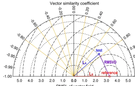
and the RMSVD are shown in Fig. 1. As for the case of two-dimensional vectors (Xu et al., 2016), the RMSLs, i.e., LA
and LB, measure the mean and variance of the lengths of vector fields AandB, respectively (Eqs. A4, A5). Rv
re-flects the pattern similarity between two vector fields. The RMSVD describes the overall difference between two vector fields. Thus, the three statistical quantities can be indicated by a single point on the VFE diagram (Fig. 1).
3 Multivariable integrated evaluation with the VFE diagram
3.1 Methodology
To evaluate model performance in terms of the simulation of multiple variables, one can group various scalar fields into a vector field and compare the constructed vector field against the observed one using the VFE diagram. For example, we can construct a vector field with temperature and precipita-tion as its x andy components, respectively. One can cer-tainly use more variables as needed to construct the vector field. Note that the statistical quantities RMSL, VSC, and RMSVD in the VFE diagram are defined in an orthogonal coordinate system in which the axes are perpendicular to each other. There is no requirement for the independence of the variables to be evaluated, e.g., temperature and precipita-tion which are represented by coordinate values of individual axes. Thus, the VFE diagram can be applied to evaluate any combination of modeled variables against corresponding ob-servational estimates. Given the differences in units and or-der of magnitude of various variables, we need to normalize all variables before grouping them into a vector field. The normalization can be done by dividing the rms value of each observational estimate as follows:
A?j= a1j
Lb1 ,a2j
Lb2
, . . ., aMj LbM
=a1j? , a?2j, . . ., a?Mj;
j =1,2, . . ., N (19)
B?j = b
1j
Lb1, b2j Lb2, . . .,
bMj LbM
=b1j? , b?2j, . . ., b?Mj;
j =1,2, . . ., N, (20)
whereLbi =
s
1 N
N
P
j=1
b2ij is the rms value for theith compo-nent of vector fieldBobtained from observational estimates. Each component of the normalized vector field is dimension-less and on the order of 1. Thus, the statistics of each compo-nent are equally important to the total statistics of the vector fields. The normalization is especially necessary when the variables are of different orders of magnitude. For example, the surface air temperature (SAT) is typically on the order of 100–101◦C, but the monthly mean precipitation rate is gen-erally on the order of 10−5–10−4mm s−1. Under this
circum-LA
LB
RMSVD Vector similarity coefficient
RMSL of vector field
Figure 1.VFE diagram for displaying multiple statistics of two vec-tor fields. The vecvec-tor similarity coefficient between two vecvec-tor fields is given by the azimuthal position of the test field. The radial dis-tance from the origin is proportional to the RMSL of the vector
field.LAandLBrepresent the RMSL of the test and reference
vec-tor fields, respectively. The RMSVD between the test and reference fields is proportional to their distance (dashed contours are given in the same units as those for the RMSL).
stance, the differences in the RMSL, VSC, and RMSVD be-tween various models would be primarily determined based on the SAT and barely impacted by the precipitation if no normalization was applied. Therefore, in terms of the MVIE of the model performance, the RMSLs, VSC, and RMSVD should be computed using the normalized vector fieldsA? andB?. As interpreted in Sect. 2, three statistical quantities in the VFE diagram represent the overall statistics across all components between two vector fields. If the vector fields are grouped by various scalar fields, the VFE diagram can summarize the three statistics of model performance in sim-ulating multiple scalar fields.
3.2 Application of multivariable integrated evaluation of model performance
Table 1.Multiple statistics of CMIP5 models in simulating surface air temperature and precipitation in terms of climatological mean state and interannual variability. Tm (Pm) is the climatological mean surface air temperature (precipitation) in summer (June–July–August). Ta (Pa) is the temporal standard deviation of summer surface air temperature (precipitation). CMIP5 simulations and three individual groups of observational datasets are compared with the ensemble mean of three groups of SAT and precipitation data observed during the period from 1961 to 2000. The rms is the ratio of modeled to observed root mean square values of the spatial pattern for each variable. CORR (RMSD) is the uncentered spatial correlation coefficient (root mean square deviation) between model and observational fields. RMSL, Rv, and RMSVD measure the statistics of two vector fields, which can represent the overall statistics of all fields (Eqs. 3, 13, 16). RMSL was shown as the ratio of model simulated RMSL to the observed RMSL. The rms_std is the standard deviation of four rms values, which describe the dispersion of rms values of Tm, Pm, Ta, and Pa (Eq. 23). MIEI is the multivariable integrated evaluation index (Eq. 24). Model performance is indicated by the color scale; lighter colors denote better model performance.
rms_std
rms
2008) and Global Precipitation Climatology Centre (GPCC) precipitation (Schneider et al., 2014). All observational data are available at 0.5◦×0.5◦ resolution. We take the average of three pairs of SAT and precipitation values as the refer-ence data in this study, unless stated otherwise. The obser-vational uncertainty can be roughly estimated by comparing each observational estimate to the reference data (Xu et al., 2016). All datasets were regridded to a common resolution of 2.5◦×2.5◦using a box-averaging (bilinear interpolation) method that re-grids data to a coarse (fine) resolution. All datasets were weighted by the area of the grid cell to make the statistics more representative for the global mean val-ues. Both the model and observational data are normalized by the rms value of each observed field before computing their statistics (Eqs. 19, 20).
Table 1 shows the various statistics of nine CMIP5 mod-els in terms of the climatological mean summer (June–July– August) SAT, precipitation, and the temporal standard de-viation of SAT and precipitation over the global land area (60◦S–60◦N). The standard deviation reflects the amplitude
of interannual variation. The models can generally well sim-ulate the climatological mean SAT characterized by the close correspondence of the rms values, high uncentered correla-tions, and small RMSDs between the model and observation. In contrast, models show a relatively poor performance in simulating other variables, i.e., climatological mean precip-itation, standard deviations of SAT and precipitation. These statistics vary from one model to the next. It is difficult to
compare the overall performance of various models because there are too many variables and models to distinguish one from another (Table 1). It is very useful to summarize the statistics of multiple variables with fewer indices, which en-ables an objective evaluation of the overall model perfor-mance in simulating multiple variables. To achieve this goal, we grouped the four normalized scalar fields into a four-dimensional vector field. Afterwards, we computed the sta-tistical quantities, i.e., RMSL, VSC, and RMSVD, with the four-dimensional vector fields derived from model and obser-vational data. As interpreted in Sect. 2, the RMSL (RMSVD) measures the overall rms values (RMSDs) of all scalar fields (Eqs. 3, 16). The VSC represents the weighted average of uncentered correlation coefficients across all scalar fields (Eq. 13). Thus, each model’s performance in simulating mul-tiple variables can be summarized by a single point that is determined by 12 statistical quantities (4 variables×3 statis-tics) derived from various scalar fields (Table 1, Fig. 2).
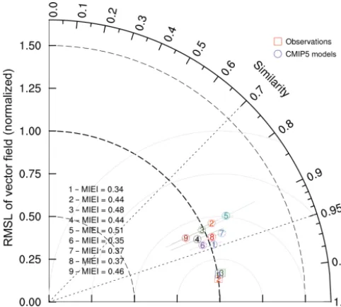
Figure 2.VFE diagram describing the normalized climatological mean SAT, precipitation, and interannual variabilities of SAT and
precipitation over a land area between 60◦S and 60◦N simulated
by nine CMIP5 models compared with three groups of SAT and precipitation data observed during the period from 1961 to 2000. The RMSL and the RMSVD have been normalized by dividing the RMSL derived from the observed data. The line segment centered at each plotted point along the azimuthal direction represents 2 stan-dard deviations of the rms values of various fields. The value of the MIEI for each model is also shown in the diagram.
values. For example, models 5 and 7 overestimate the RM-SLs of the four-dimensional vector fields, suggesting that both models generally overestimate the rms values of the four scalar fields. This can also be confirmed by Table 1, as model 5 clearly overestimates the rms values of Ta (1.43) and Pa (1.19) and slightly underestimates the rms values of Tm (0.99) and Pm (0.94). Model 7 overestimates all rms values (1.06, 1.09, 1.14, and 1.07) of the four variables. Thus, the RMSL of a constructed vector field can reasonably represent the overall performance of a model in reproducing rms values of multiple scalar fields. In contrast, model 9 clearly under-estimates the RMSL of the vector field (Fig. 2). Correspond-ingly, three out of the four rms values of scalar fields are smaller than 1 for model 9 (Table 1). Similarly, the RMSVD between two vector fields can also reasonably represent the overall RMSDs of multiple scalar fields as shown in Fig. 2 and Table 1. Thus, one can evaluate the model performance in simulating multiple variables with three statistical quanti-ties. The three statistical quantities represent different aspects of model performance, the knowledge of which can provide a more comprehensive model evaluation. The VFE diagram can clearly illustrate to what extent the overall RMSDs of various scalar fields (represented by the RMSVD) are at-tributable to the systematic difference in rms values
(repre-sented by the RMSL) and how much is due to the poor pat-tern similarities (represented byRv).
Note that model performance does not change monoton-ically with the increase or decrease in rms values. Specif-ically, model performance improves as the normalized rms values approach 1 but decreases as the normalized rms val-ues approach either zero or infinity. As defined in Eq. (3), the RMSL being equal to the sum of rms values of all com-ponents of a vector field. Thus, even if the modeled RMSL is equal to the observed one, it does not necessarily suggest that the model well reproduces the rms values of various scalar fields. This conclusion may result from the cancella-tion between the overestimated and the underestimated rms values. For example, as shown in Table 1, model 3 overesti-mates the rms values of Tm (1.05) and Ta (1.26) but underes-timates the rms values of Pm (0.80) and Pa (0.77). However, the RMSL (0.99) is almost consistent with the observational estimate. Under such a circumstance, the RMSL misrepre-sents the model performance in simulating rms values of var-ious scalar fields. To mitigate this shortcoming, one can add a line segment centered at each plotted point along the az-imuthal direction (Fig. 2). The length of the line segment is equal to twice the standard deviation of rms values of mul-tiple scalar fields. Thus, the length of the line segment can measure the dispersion of various rms values relative to their mean. A shorter line indicates that the rms values are close to the mean. In contrast, a longer line segment indicates that the rms values are spread out over a wider range. To measure the accuracy of modeled rms values to that of those observed, one can use the root mean square deviation of the rms values of various variables:
RMSD2L= 1
M M
X
i=1
L?ai−L?bi2, (21)
where L?ai= 1
Lbi
s
1 N
N
P
j=1
aij2 and L?bi= 1
Lbi
s
1 N
N
P
j=1 b2ij are the rms values of the ith normalized component of vector fieldsAandB, respectively. With the support of Eq. (6), we haveL?bi=1 for alli(1≤i≤M). The RMSD2Lcan be fur-ther written as
RMSD2L= 1
M M
X
i=1
L?ai−12
= 1
M M
X
i=1
L?ai2− 2
M M
X
i=1 L?ai+1
= 1
M M
X
i=1 L?
a+L?ai
02 −2L?
a+1
=L? a 2
+ 1
M M
X
i=1
L?ai02−2L? a+1
= L? a−1
2
whereL?
a, andL?ai
0
are the mean and anomaly ofL?ai, respec-tively. The rms value ofL?ai0is written as follows:
σrms=
1
M M
X
i=1 L?ai02
!12
. (23)
σrms is the centered rms value or the standard deviation of
L?ai. Thus, the RMSDLcan be decomposed into the mean
er-ror and the variance of rms values of normalized scalar fields (Eq. 22). RMSDLmeasures the overall deviation of modeled
rms values from the observed ones. The modeled rms values of various scalar fields are exactly equal to the corresponding observed ones only when the RMSDLis equal to 0.
3.3 Multivariable integrated evaluation index for model performance
In general, the model results get closer to the observational estimate as the RMSVD decreases. It is noteworthy that for a given VSC at a relatively low value, the RMSVD does not strictly decrease monotonically as the simulated RMSL ap-proaches the observed one (Fig. 3). For example, model B shows the same VSC as that of model A but a smaller bias in the RMSL, which suggest that model B performs better than model A. However, the RMSVD is greater in model B than in model A (Fig. 3). Thus, the decrease in the RMSVD may not necessarily indicate an improvement in model performance. On the other hand, given the drawback of the RMSL in mea-suring the accuracy of rms values, the model skill score, de-fined based on the RMSL and VSC in Xu et al. (2016), is also not well suited for measuring the model performance in sim-ulating multiple scalar fields. To better measure model per-formance, we define a multivariable integrated evaluation in-dex (MIEI) based on the VFE diagram (Fig. 3):
MIEI2=BC2+BG2.
Based on the law of cosines, we have BG2=2−2Rv.
Thus, the MIEI can be written as
MIEI2=RMSD2L+2(1−Rv)
=σrms2 + L? a−1
2
+2(1−Rv) . (24)
Clearly, the MIEI takes both the amplitudes and pattern sim-ilarities of various variables into account and therefore can provide a comprehensive evaluation of model performance (Eq. 24). In contrast to the RMSVD, the MIEI satisfies the monotonic property of an index with respect to model perfor-mance. Specifically, for any givenσrmsandL?a, the MIEI
de-creases monotonically with the increase inRv. For any given σrms andRv, the MIEI decreases monotonically as L?a
ap-proaches 1. For any given L?
a andRv, the MIEI decreases
A B
RMSDL
D C
G MIEI
RMSL of vector field (normalized)
Figure 3.Schematic diagram displaying the relationship between
the RMSVD, RMSDL, and MIEI. The points A, B, and D represent
different models. The RMSDLmeasures the overall difference
be-tween the modeled rms values and the observed ones. The line seg-ment BC is vertical with respect to the VFE diagram. The length of line segment BG is determined based on the vector field similarity, which measures the overall pattern similarity of various scalar fields relative to the observed ones. Thus, the MIEI index takes both the pattern similarities and the rms values of various scalar fields into account.
monotonically with the decrease inσrms. The MIEI is equal
to 0 only whenσrms=0,L?a=1, andRv=1, which define
a perfect model. In other words, modeled multiple fields are exactly the same as the observed ones when the MIEI is equal to 0.
mul-tiple statistics, i.e., pattern similarity, rms values and their variances, and RMSVD.
The issue of how to take the observational uncertainties into account is of particular importance in model evaluation and ranking, especially when more and more observational datasets provide estimates of the observational uncertainty. The statistics derived from each group of observational esti-mates are also shown in Table 1, which can roughly quantify the observational uncertainties and its impact on model eval-uation. Generally, the colors are clearly lighter for the statis-tics of individual observed variables in contrast to the mod-eled variables (Table 1). This indicates that the observational uncertainties are relatively small and should have less im-pact on the evaluation of model performance. To further quantify the impacts of observational uncertainty on rank-ing model performance, we calculate the MIEIs of various climate models by taking each group of observational esti-mates as the reference data. Three groups of observational es-timates generate three groups of MIEIs. Afterwards, we cal-culate Spearman’s rank correlation coefficient of each group of MIEIs with those derived from models and the ensemble mean of multiple observational estimates. The Spearman’s rank correlation coefficients are 0.996, 0.996, and 0.904, re-spectively, suggesting that the ranks are very close to each other no matter which group of observational estimates is used as reference data. Thus, the observational uncertainty should have less impact on ranking model performance in this case. One can use the average of Spearman’s rank cor-relation coefficients to quantify the consistency of various ranks when a number of observational estimates are avail-able.
4 Summary and discussion
The MVIE method proposed here provides a concise way of representing the multiple statistics of multiple fields on a two-dimensional plot, i.e., the VFE diagram. The VFE dia-gram includes three statistical quantities, i.e., RMSL, VSC, and RMSVD, representing different aspects of model per-formance. Specifically, the RMSL (RMSVD) represents the total mean value and variance (total RMSDs) of all scalar fields. The VSC measures the overall pattern similarity across all scalar fields. As shown in the example, each of the three statistical quantities can reasonably represent the cor-responding statistics of multiple scalar fields. Moreover, the VFE diagram can illustrate how much the overall RMSD of various fields is attributable to the difference in rms values and how much is due to poor pattern similarity. Thus, one can summarize multiple statistics of multiple variables for various models in a diagram and facilitate the intercompari-son of model performance in simulating multiple variables. The MVIE method can be applied to spatial and/or temporal fields. It can also simultaneously evaluate various temporal variabilities simulated by models, e.g., climatological mean
state and the amplitude of interannual variability as shown in Sect. 3.2. Based on the VFE diagram, we also developed a MIEI which takes the amplitude and pattern similarity of multiple fields into account. The MIEI satisfies the criterion that a model performance index should vary monotonically as the model performance improves. The MIEI provides a more concise evaluation than the VFE diagram of model per-formance in simulating multiple fields.
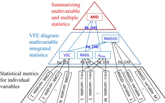
The statistical metrics presented in this paper can be di-vided into three different levels and their relationships are summarized in a pyramid chart (Fig. 4). The first level of metrics, i.e., correlation coefficient, rms value, and RMSD, measures model performance in terms of individual vari-ables. These metrics can be illustrated by a table of met-rics (Table 1), which can provide detailed information on model performance in simulating individual variables but cannot give a quantitative evaluation of the overall model performance in simulating multiple fields. The second level of metrics, i.e., the VSC, RMSL, standard deviation of rms values, and RMSVD, is derived from the first level of met-rics and represents the overall statistics of multiple variables. The second level of metrics can be presented as a VFE dia-gram, which provides an integrated evaluation of model per-formance in terms of simulating multiple fields. The MIEI belongs to the third level of metrics, which is defined based on the VFE diagram. The MIEI further summarizes the three statistical quantities of the VFE diagram into a single in-dex and can be used to rank the performance of various cli-mate models. A higher level of metrics provides a more con-cise evaluation of model performance compared to a lower level of metrics, which facilitates model intercomparison. Unavoidably, the higher level of metrics loses detailed statis-tical information in contrast to the lower level of metrics. To provide a more comprehensive evaluation of model perfor-mance, one can show the VFE diagram together with a table of statistical metrics (Table 1) or other model performance metrics as needed.
rm s :
va
ria
ble
1
rm s :
va
ria
ble
2
rm s :
va
ria
ble
M
…
VSC RMSL
RMSVD
MIEI
Statistical metrics for individual variables
VFE diagram: multivariable integrated statistics
Summarizing multivariable and multiple statistics
Eq. (13) Eq. (3) Eq. (23) Eq. (16)
Eq. (24)
Eq. (18)
rm s
Figure 4.Pyramid chart showing the relationship between three levels of metrics. The first level of metrics, i.e., correlation coefficient (CORR), rms value, and RMSD, measures the model performance in terms of individual variables. The second level of metrics, i.e., VSC,
RMSL, standard deviation of rms values (σrms), and RMSVD, is derived from the first level of metrics and summarizes the overall
perfor-mance of a climate model in simulating multiple fields. The MIEI further summarizes the VSC, RMSL, andσrms2 into a single index to rank
various climate models in terms of simulating multiple fields.
been argued that the uncentered statistics are better suited for detection because they incorporate the response of the mean value. In contrast, the centered statistics are more appropri-ate for attribution because they better measure the similarity between spatial patterns (Hegerl et al., 2001). The VFE dia-gram provides us flexibility in model evaluation. In terms of model evaluation aimed at a detection study, one can com-pute the uncentered statistics with full fields. In contrast, one can use centered statistics by computing the statistical quan-tities with vector anomaly fields if an attribution study is the major concern of the model evaluation.
In practice, one may want to weight different fields based on their relative importance. If some variables to be evalu-ated are dependent on each other, e.g., skin temperature and surface air temperature, one may also want to weight these variables properly because the dependent variables contain redundant information. Otherwise, the evaluation of equally weighted variables may overestimate the importance of the dependent variables. Determining the weight coefficient de-pends on the application and therefore is beyond the scope of this study. Here, we only discuss how the weight can be considered in the multivariable integrated evaluation (Ap-pendix B). The MVIE method presented in this study re-quires the normalization of each modeled and observed vari-able by dividing the corresponding rms value of the observed variable (Eqs. 19, 20). Therefore, one should weight differ-ent variables after the normalization (Eqs. B1, B2); otherwise the normalization process will remove the weight coefficient. Weighting each normalized field leads to a quadratic weight-ing of the quadratic rms values, quadratic RMSDs, and cor-relation coefficients (Eqs. B1, B5, B8, B11).
The VFE diagram and MIEI may also provide some guidance in weighting various climate models to constrain future climate projection. A recent study suggested that model weighting should take both model performance and model interdependencies into account to improve climate projections (Knutti et al., 2017). The VFE diagram can sum-marize model performance in terms of multiple statistics of multiple fields, on one hand. On the other hand, the VFE diagram can also clearly show the differences between model and observation as well as the differences between various models. This information provided by the VFE di-agram may be used in weighting climate models, which war-rant further studies.
Code availability. The code used in the production of Fig. 2 and Table 1 is available in the Supplement.
Appendix A: Decomposition of RMSL, VSC, and RMSVD
To further interpret the RMSL, VSC, and RMSVD, we break down the full vector fields A and B into the mean and anomaly:
Aj =A+A0j=a1+a1j0 , a2+a02j,· · ·, aM+a0Mj;
j =1,2, . . ., N Bj=B+Bj0 =
b1+b01j, b2+b2j0 ,· · ·, bM+bMj0
;
j =1,2, . . ., N,
where
A=(a1, a2,· · ·, aM) ,
B= b1, b2,· · ·, bM,
A0j =a1j0 , a02j,· · ·, a0Mj, Bj0 =b1j0 , b02j,· · ·, b0Mj,
ai=
1
N N
X
j=1
aij; i=1,2, . . ., M
bi=
1
N N
X
j=1
bij; i=1,2, . . ., M
aij0 =aij−ai; i=1,2, . . ., M b0ij=bij−bi; i=1,2, . . ., M.
The squared RMSL of vector fieldAis written as follows:
L2A= 1
N N
X
j=1
Aj 2 = 1 N N X
j=1 M
X
i=1
ai+aij0 2
= 1
N N
X
j=1 M
X
i=1 ai2+
1
N N
X
j=1 M
X
i=1
aij0 2+ 1
N N
X
j=1 M
X
i=1
2aiaij0 .
Given
N
P
j=1
aij0 =0,L2Acan be written as
L2A= 1
N N
X
j=1 M
X
i=1 ai2+
1
N N
X
j=1 M
X
i=1 aij0 2
= 1
N N
X
j=1
A 2 + 1 N N X
j=1
A 0 j 2
=L2 A+L
2
A0, (A1)
where
LA= 1
N N
X
j=1
A
2
!12
=A=
M
X
i=1 ai2
!12
(A2)
is the RMSL of the mean vector field,
LA0 = 1 N
N
X
j=1
A 0 j 2! 1 2 = M X
i=1 σai2
!12
(A3)
is the RMSL of the vector anomaly field, and
σai=
1
N N
X
j=1 a0ij2
!12
; i=1,2, . . ., M
is the centered rms value (or standard deviation) of theith component of vector fieldA.
Equation (A1) can be written as
L2A=L2 A+L
2 A0=
M
X
i=1
ai2+σai2
. (A4)
The RMSL of vector fieldA,LA, measures the overall mean value and variance of all components of the vector field.
Similarly, we have
L2B=L2 B+L
2 B0=
M
X
i=1
bi2+σbi2, (A5)
where
σbi= 1
N N
X
j=1 bij0 2
!12
; i=1,2, . . ., M
is the centered rms value (or standard deviation) of theith component of vector fieldB.
With the support of Eq. (13), the VSC can be written as
Rv=
1
N LALB N
X
j=1 M
X
i=1
ai+aij0 bi+bij0
= 1
N LALB N
X
j=1 M
X
i=1
aibi+aibij0 +biaij0 +a
0 ijb 0 ij = 1
N LALB M
X
i=1 N
X
j=1 aibi+
N
X
j=1 aibij0 +
N
X
j=1 bia0ij+
N
X
j=1 a0ijb0ij
!
.
Given that
N
P
j=1 a0ij=
N
P
j=1
b0ij=0 for alli(1≤i≤M), we ob-tain
Rv= 1
N LALB M
X
i=1 N
X
j=1 aibi+
N
X
j=1 aij0 b0ij
!
=LALB
LALB
Rv+LA0LB0
LALB
where
Rv= 1
N LALB N
X
j=1 M
X
i=1
aibi= 1
LALB M
X
i=1
aibi (A7)
Rv0= 1
N LA0LB0 N
X
j=1 M
X
i=1
aij0 b0ij. (A8)
Given the Cauchy–Schwarz inequality, Eq. (A7) can be rewritten as
Rv2= M
P
i=1 aibi
2
LALB2
≤
M
P
i=1 ai2
M
P
i=1 bi
2
LALB2
= L
2 AL
2 B
LALB2
=1.
Rv reaches its maximum value of 1 when ab1 1
=a2 b2
=. . .=
aM bM
>0. In contrast, Rv reaches its minimum value of −1
when a1 b1
=a2 b2
=. . .=aM
bM <0. Rv measures the extent of
correlation between modeled and observed mean values across all components of two vector fields.
Equation (A8) can be rewritten as
Rv0= 1
N LA0LB0 N
X
j=1 M
X
i=1 a0ijb0ij σaiσbi
σaiσbi
= 1
N LA0LB0 M
X
i=1 N
X
j=1 a0ijb0ij σaiσbi
σaiσbi
= 1
LA0LB0 M
X
i=1 σaiσbi
1
N N
X
j=1 aij0 bij0 σaiσbi
!
= 1
LA0LB0 M
X
i=1
σaiσbiri, (A9)
whereσai andσbi are the centered rms values (or standard
deviation) of theith component of vector fieldAandB, re-spectively.
ri =
1
N N
X
j=1 aij0 b0ij σaiσbi
represents the centered correlation coefficients between the
ith paired components of vector fieldsAandB.Rv0 can be interpreted as a weighted average of the centered correlation coefficients across all paired components between two vector fields. The weight coefficients are proportional to the product of standard deviations between paired variables. Clearly, the VSC is simultaneously determined based on the correlation of various mean fields and the overall correlation of anomaly fields across all paired components between two vector fields (Eqs. A6, A7, A9).
The RMSVD between two vector fields can also be repre-sented by the mean and anomaly fields:
RMSVD2= 1
N N
X
j=1
Aj−Bj
2 = 1 N N X
j=1 M
X
i=1
ai+a0ij−bi−b0ij
2
= 1
N M
X
i=1 N
X
j=1
ai−bi+a0ij−b0ij 2
= 1
N M
X
i=1 N
X
j=1
ai−bi 2
+
N
X
j=1
aij0 −bij0 2
+2 ai−bi
N
X
j=1
aij0 −b0ij
!
.
Given that
N
P
j=1 a0ij=
N
P
j=1
b0ij=0 for alli(1≤i≤M), we ob-tain
RMSVD2= 1
N M
X
i=1 N
X
j=1
ai−bi2+
N
X
j=1
aij0 −bij0
2 ! = 1 N N X
j=1 M
X
i=1
ai−bi 2
+ 1
N N
X
j=1 M
X
i=1
aij0 −b0ij2
= 1
N N
X
j=1
A−B
2 + 1 N N X
j=1
A
0
j−B
0 j 2
=(RMSVDm)2+(RMSVDa)2, (A10) where
(RMSVDm)2=
M
X
i=1
ai−bi2 (A11)
is the RMSVD between mean vector fieldsAandB, which represents the mean difference of all fields.
(RMSVDa)2=
M
X
i=1
1
N N
X
j=1
aij0 −b0ij2
!
=
M
X
i=1
RMSD0i2 (A12)
is the centered RMSVD between two vector fields, which represents the overall RMSD across all paired components of vector anomaly fieldsA0 andB0. From the viewpoint of MVIE, the RMSVD can be interpreted as the overall mean difference of all fields plus the overall RMSD of all anomaly fields.
evaluation. The statistical quantities, i.e., RMSL, VSC, and RMSVD, computed based on the full vector fields represent the uncentered pattern statistics, which include the statistics from both the mean and anomaly fields. Alternatively, three statistics can also be computed based on the anomaly fields, yielding centered statistics, which only measure the anomaly fields. The full vector fields should be used if both the mean and anomaly need to be evaluated. In contrast, the anomaly vector fields should be used if anomaly fields are the primary concern.
Appendix B: Weighted multivariable integrated evaluation with VFE diagram
In terms of model evaluation, one may care for some vari-ables more than other varivari-ables, although all varivari-ables are of great concern. In such a circumstance, it would be use-ful to weight different variables to make the VSC, RMSL, and RMSVD more sensitive to some variables than to others. Without loss of generality, the weighted- and normalized-vector fields AwandBw can be written as a pair of vector sequences:
Awj =w·A?j =
w1a?1j, w2a?2j, . . ., wMaMj?
;
j =1,2, . . ., N (B1)
Bwj =w·B?j=w1b1j? , w2b2j? , . . ., wMbMj?
;
j =1,2, . . ., N, (B2)
whereaij? andbij? (1≤i≤M)are the same as in Eqs. (19) and (20).wi is the weight coefficient for theith component
of the vector field and satisfies the constraint
M
X
i=1
wi =M.
Note that the weighting should be applied to the normalized model and observational data (Eqs. B1, B2). Otherwise, the normalization would remove the weight coefficient (Eqs. 19 and 20). Based on Eq. (3), the square of the RMSL of the normalized vector fieldA?can be written as follows:
L?A2=
M
X
i=1
L?ai2, (B3)
whereL?ai= 1
N N
P
j=1 aij?2
!12
denotes the rms value of theith component of the normalized vector fieldA?. Similarly, the quadratic RMSL of weighted- and normalized-vector fields can be written as follows:
LwA2=
M
X
i=1
Lwai2, (B4)
whereLwai= 1
N N
P
j=1 w2iaij?2
!12
=wiL?ai is the rms value of
theith component of vector fieldAw. With the support of Eqs. (B1), (B3), and (B4), it is easy to obtain
LwA2=
M
X
i=1 Lwai2=
M
X
i=1
wi2L?ai2. (B5)
The RMSL of vector fieldAw is determined based on the weighted rms values across all components of the vector field. The contribution of the ith rms value, L?ai, to the quadratic RMSL of the vector field is weighted byw2i. The rms value accounts for more of the RMSL when its weight coefficient is greater.
Based on Eq. (16), the square of the RMSVD between nor-malized vector fieldsA?andB?can be written as follows:
RMSVD?2=
M
X
i=1
RMSD?i2, (B6)
where RMSDi= N1 N
P
j=1
aij? −b?ij 2!
1 2
is the RMSD of theith paired components between normalized vector fields A? andB?. Similarly, the square of the RMSVD between weighted vector fieldsAwandBwcan be written as follows:
RMSVDw2=
M
X
i=1
RMSDwi 2
. (B7)
RMSDwi = 1
N N
P
j=1
wiaij? −wibij?
2 !12
is the RMSD of the
ith paired components between weighted vector fields Aw andBw. With the aid of Eqs. (B1), (B2), (B6), and (B7), we obtain
RMSVDw2 =
M
X
i=1
RMSDwi 2 =
M
X
i=1
wi2RMSD?i2. (B8)
The RMSVD between two vector fields is determined based on the weighted RMSDs across all paired components of two vector fields. The contribution of theith RMSD to the quadratic RMSVD between two vector fields is weighted by
w2i.
Based on Eq. (13), the VSC between normalized vector fieldsA?andB?can be written as follows:
Rv?= 1
L?A·L?B M
X
i=1
L?aiL?biRui? , (B9)
whereL?ai= 1
N N
P
j=1 aij?2
!12
and L?bi= 1
N N
P
j=1 b?ij2
fieldsAandB, respectively.Rui? = 1
N N P
j=1
a?
ijb?ij
L?aiL?bi is the
uncen-tered correlation coefficient for theith components between two vector fields. Similarly, the VSC between weighted fields can be rewritten as
Rvw= 1
LwA·LwB M
X
i=1
LwaiLwbiRuiw, (B10)
whereLwai,Lwbi, andRuiw are the same asL?ai,L?bi, andRui?, respectively, except they are computed based on the weighted vector fields Aw andBw. With the aid of Eqs. (B1), (B2), (B9), and (B10), we obtain
Rvw= 1
LwA·LwB M
X
i=1
wi2L?aiL?biRui?. (B11)
The Supplement related to this article is available online at https://doi.org/10.5194/gmd-10-3805-2017-supplement.
Author contributions. ZX devised the evaluation method and wrote the paper. All of the authors discussed the results and commented on the paper.
Competing interests. The authors declare that they have no conflict of interest.
Acknowledgements. We acknowledge the World Climate Research Programme’s Working Group on Coupled Modelling, which is responsible for CMIP, and we thank the climate modeling groups for producing and making available their model output. The study was supported jointly by the National Key Research and Development Program of China (2016YFA0600403), the Major Research Plan of the National Science Foundation of China (91637103), and the National Science Foundation of China Grant (41675080, 41675105). This work was also supported by the Jiangsu Collaborative Innovation Center for Climate Change.
Edited by: Klaus Gierens
Reviewed by: two anonymous referees
References
Chen, H. and Sun, J.: Assessing model performance of climate extremes in China: an intercomparison between CMIP5 and CMIP3, Climatic Change, 129, 197–211, 2015.
Eyring, V., Gleckler, P. J., Heinze, C., Stouffer, R. J., Taylor, K. E., Balaji, V., Guilyardi, E., Joussaume, S., Kindermann, S., Lawrence, B. N., Meehl, G. A., Righi, M., and Williams, D. N.: Towards improved and more routine Earth system model evaluation in CMIP, Earth Syst. Dynam., 7, 813–830, https://doi.org/10.5194/esd-7-813-2016, 2016.
Fan, Y. and van den Dool, H.: A global monthly land surface air temperature analysis for 1948–present, J. Geophys. Res., 113, D01103, https://doi.org/10.1029/2007JD008470, 2008. Fu, C., Wang, S., Xiong, Z., Gutowski, W. J., Lee, D.-K.,
McGre-gor, J. L., Sato, Y., Kato, H., Kim, J.-W., and Suh, M.-S.: Re-gional Climate Model Intercomparison Project for Asia, B. Am. Meteorol. Soc., 86, 257–266, 2005.
Giorgi, F. and Gutowski, W. J.: Regional Dynamical Downscaling and the CORDEX Initiative, Annu. Rev. Environ. Res., 40, 467– 490, 2015.
Gleckler, P. J., Taylor, K. E., and Doutriaux, C.: Performance metrics for climate models, J. Geophys. Res., 113, D06104, https://doi.org/10.1029/2007JD008972, 2008.
Harris, I., Jones, P. D., Osborn, T. J., and Lister, D. H.: Up-dated high-resolution grids of monthly climatic observations – the CRU TS3.10 Dataset, Int. J. Climatol., 34, 623–642, https://doi.org/10.1002/joc.3711, 2014.
Hegerl, G. C., Zwiers, F. W., Allen, M. R., and Marengo J.: De-tection of Climate Change and Attribution of Causes, in: Cli-mate Change 2001: The Scientific Basis. Contribution of Work-ing Group I to the Third Assessment Report of the Intergovern-mental Panel on Climate Change, edited by: Houghton, J. T., Ding, Y., Griggs, D. J., Noguer, M., van der Linden, P. J., Dai, X., Maskell, K., and Johnson, C. A., Cambridge University Press, Cambridge, UK and New York, NY, USA, 881 pp., 2001. IPCC: Managing the Risks of Extreme Events and Disasters to
Ad-vance Climate Change Adaptation. A Special Report of Work-ing Groups I and II of the Intergovernmental Panel on Climate Change, edited by: Field, C. B., Barros, V., Stocker, T. F., Qin, D., Dokken, D. J., Ebi, K. L., Mastrandrea, M. D., Mach, K. J., Plattner, G.-K., Allen, S. K., Tignor, M., and Midgley, P. M., Cambridge University Press, Cambridge, UK, and New York, NY, USA, 582 pp., 2012.
IPCC: Climate Change 2013: The Physical Science Basis. Con-tribution of Working Group I to the Fifth Assessment Report of the Intergovernmental Panel on Climate Change, edited by: Stocker, T. F., Qin, D., Plattner, G.-K., Tignor, M., Allen, S. K., Boschung, J., Nauels, A., Xia, Y., Bex, V., and Midgley, P. M., Cambridge University Press, Cambridge, UK and New York, NY, USA, 1535 pp., 2013.
Knutti, R., Sedláˇcek, J., Sanderson, B. M., Lorenz, R., Fischer, E. M., and Eyring V.: A climate model projection weighting scheme accounting for performance and interdependence, Geophys. Res. Lett., 44, 1909–1918, https://doi.org/10.1002/2016GL072012, 2017.
Legates, D. R. and Davis, R. E.: The continuing search for an anthropogenic climate change signal: limitations of correlation based approaches, Geophys. Res. Lett., 24, 2319–2322, 1997. Mearns, L. O., Gutowski, W. J., Jones, R., Leung, L.-Y., McGinnis,
S., Nunes, A. M. B., and Qian, Y.: A regional climate change assessment program for North America, Eos, Trans. Amer. Geo-phys. Union, 90, 311–312, 2009.
Murphy, A. H.: Skill scores based on the mean square error and their relationships to the correlation coefficient, Mon. Weather Rev., 116, 2417–2424, 1988.
Pierce, D. W., Barnett, T. P., Santer, B. D., and Gleckler, P. J.: Selecting global climate models for regional climate change studies, P. Natl. Acad. Sci. USA, 106, 8441–8446, https://doi.org/10.1073/pnas.0900094106, 2009.
Pincus, R., Batstone, C. P., Hofmann, R. J. P., Taylor, K. E., and Gleckler, P. J.: Evaluating the present-day simulation of clouds, precipitation, and radiation in climate models, J. Geophys. Res., 113, D14209, https://doi.org/10.1029/2007JD009334, 2008. Radi´c, V. and Clarke, G. K. C.: Evaluation of IPCC models’
per-formance in simulating late-twentieth-century climatologies and weather patterns over North America, J. Climate, 24, 5257–5274, 2011.
Schneider, U., Becker, A., Finger, P., Meyer-Christoffer, A., Rudolf, B., and Ziese, M.: GPCC Full Data
Reanaly-sis Version 6.0 at 0.5◦: Monthly Land-Surface Precipitation
from Rain-Gauges built on GTS-based and Historic Data, https://doi.org/10.5676/DWD_GPCC/FD_M_V7_050, 2011. Schneider, U., Becker, A., Finger, P., Meyer-Christoffer, A., Ziese,
quantifying the global water cycle, Theor. Appl. Climatol., 115, 15–40, https://doi.org/10.1007/s00704-013-0860-x, 2014. Taylor, K. E.: Summarizing multiple aspects of model performance
in a single diagram, J. Geophys. Res.-Atmos., 106, 7183–7192, 2001.
Taylor, K. E., Stouffer, R. J., and Meehl G. A.: An Overview of CMIP5 and the experiment design, B. Am. Meteorol. Soc., 93, 485–498, https://doi.org/10.1175/BAMS-D-11-00094.1, 2012. van der Linden, P. and Mitchell, J. F. B. (Eds.): ENSEMBLES:
Climate change and its impacts: Summary of research and re-sults from the ENSEMBLES project. Met Office Hadley Centre, FitzRoy Road, Exeter, UK, 160 pp., 2009.
Willmott, C. J. and Matsuura, K.: Terrestrial Air Temperature and Precipitation: Monthly and Annual Time Series (1950–1999), available at: http://climate.geog.udel.edu/~climate/html_pages/ README.ghcn_ts2.html (last access: 16 October 2017), 2001. Xu, Z., Hou, Z., Han, Y., and Guo, W.: A diagram for