TempestExtremes: a framework for scale-insensitive pointwise feature tracking on unstructured grids

(1)

Geosci. Model Dev., 10, 1069–1090, 2017 www.geosci-model-dev.net/10/1069/2017/ doi:10.5194/gmd-10-1069-2017

TempestExtremes: a framework for scale-insensitive pointwise

feature tracking on unstructured grids

Paul A. Ullrich1_{and Colin M. Zarzycki}2

1_{Department of Land, Air and Water Resources, University of California, Davis, One Shields Ave., Davis, CA 95616, USA} 2_{National Center for Atmospheric Research, Boulder, CO, USA}

Correspondence to:Paul A. Ullrich ([email protected]) Received: 17 August 2016 – Discussion started: 26 September 2016

Revised: 4 January 2017 – Accepted: 8 January 2017 – Published: 7 March 2017

Abstract.This paper describes a new open-source software framework for automated pointwise feature tracking that is applicable to a wide array of climate datasets using ei-ther structured or unstructured grids. Common climatologi-cal pointwise features include tropiclimatologi-cal cyclones, extratropiclimatologi-cal cyclones and tropical easterly waves. To enable support for a wide array of detection schemes, a suite of algorithmic ker-nels have been developed that capture the core functionality of algorithmic tracking routines throughout the literature. A review of efforts related to pointwise feature tracking from the past 3 decades is included. Selected results using both re-analysis datasets and unstructured grid simulations are pro-vided.

1 Introduction

Automated pointwise feature tracking is an algorithmic tech-nique for objective identification and tracking of meteoro-logical features, such as extratropical cyclones, tropical cy-clones and tropical easterly waves, and has emerged as an important and desirable data processing capability in climate science. Software tools for feature tracking – typically re-ferred to as “trackers” – have been employed to evaluate model performance and answer pressing scientific questions regarding anticipated changes in atmospheric features under climate change. Exploration of tracker literature has exposed a breadth of potential techniques that have been applied to climate datasets with varied spatial resolution and temporal frequency (a comprehensive review of the tracking literature can be found in Appendices A, B and C). Nonetheless, the definition of an optimal objective criteria for key atmospheric

features has eluded development, and ambiguity in the for-mal definition of these features suggests that there may be no singular criteria capable of both perfect detection and zero false alarm rate. Further, as observed by Walsh et al. (2007) and Horn et al. (2014) for tropical cyclones and Neu et al. (2013) for extratropical cyclones, feature tracking schemes can produce wildly varying results depending on the specific choice of threshold variables and values. Therefore, we argue that uncertainties associated with objective tracking criteria should be addressed with an ensemble of detection thresholds and variables, whereas blind application of singular tracking formulations should be avoided. To this end, it is the goal of this paper to review the vast literature on trackers and use this information to inform the development of a unified frame-work (TempestExtremes) that enables a variety of tracking procedures to be quickly and easily applied across arbitrary spatial resolution and temporal frequency. This paper focuses largely on the technical aspects of pointwise feature tracking, but sets the stage for future studies on parameter sensitivity and optimization.

Most algorithmic Lagrangian trackers of pointwise fea-tures (such as cyclones and eddies) share a common proce-dure:

1. They must identify an initial set of candidate points by searching for local extrema. Local extrema can be fur-ther specified, for instance, by requiring that they be suf-ficiently anomalous when contrasted with their neigh-bors. For most cyclonic structures, either minima in the sea level pressure field or maxima in the absolute value of the relative vorticity are used.

(2)

2. They must eliminate candidate points that do not satisfy a prescribed set of thresholds. For instance, tropical cy-clones typically require the presence of an upper-level warm core that is sufficiently near the sea level pressure minima that defines the storm center. Additional crite-ria, such as a minimum threshold on relative vorticity, can be used to eliminate spurious detections.

3. They must connect candidate points together in time (re-ferred to as “stitching”) to generate feature paths, elimi-nating paths that are of insufficient length or do not meet additional criteria.

Although the actual implementations of this procedure does vary throughout the literature, a review of this material re-veals several core algorithms (kernels) that are common across implementations. Based on our analysis, the five most commonly employed kernels are

– computation of anomalies in a data field from a spatially averaged mean;

– identification of local extrema in a given 2-D data field (for instance, sea level pressure minima);

– determination of whether a closed contour exists in a data field around a particular point;

– determination of whether, in the neighborhood of a par-ticular point, a data field satisfies a given threshold; and – stitching of candidates from sequential time slices to

build feature tracks.

The development of a robust implementation of these five kernels will be the focus of the remainder of this paper.

Feature tracking that is robust across essentially arbitrary datasets requires some additional considerations. Detection criteria and thresholds for tracking are often tuned based on the characteristics of a particular dataset, such as temporal resolution, spatial resolution and regional coverage. Unfor-tunately, this has led to an abundance of schemes that often cannot be directly compared, or applied in a more general context. To this end, we focus on kernels that are insensitive to the characteristics of the input data. For instance, averag-ing or searchaverag-ing over a discrete number of grid points around each candidate (a common approach) is incompatible with scale insensitivity since the physical search radius would be dependent on the spatial resolution of the data. Identifica-tion of local extrema is also a resoluIdentifica-tion-sensitive procedure, since the number of extrema will often scale with the num-ber of spatial data points; however, a closed contour criteria based on a physical distance is largely resolution insensitive. To achieve robust applicability, a general framework should

– use great-circle arcs for all distance calculations (this avoids issues associated with latitude–longitude dis-tance that emerges near the poles);

– support structured and unstructured grids (this elimi-nates the need for post-processing of large native grid output files and enables detection and characterization simultaneous with the model execution);

– not contain hard-coded variable names, so as to ensure robust applicability across reanalysis datasets and appli-cability to a variety of problems; and

– allow for easy intercomparison of detection schemes by enabling detection criteria and thresholds that are com-pactly specified on the command line.

Well-known automated software trackers include TRACK (Hodges, 1994, 1995, 2015) and the Geophysical Fluid Dynamics Laboratory (GFDL) TSTORMS package (Vitart et al., 1997; Zhao et al., 2009). Both of these software pack-ages have been used extensively to examine pointwise fea-tures in the atmosphere, but do not completely satisfy the four requirements above.

The remainder of the paper is organized as follows: Sect. 2 describes the algorithms and kernels that have been imple-mented in the TempestExtremes software framework. Se-lected examples of tropical cyclone, extratropical cyclone and tropical easterly wave detection are then provided in Sect. 3, followed by conclusions in Sect. 4. The appen-dices provide a review of relevant literature on pointwise fea-ture trackers of extratropical cyclones (Appendix A), tropi-cal cyclones (Appendix B) and tropitropi-cal easterly waves (Ap-pendix C). A technical guide to the use of the Tempes-tExtremes tools DetectCyclonesUnstructured and StitchNodesis provided in Appendices D and E. Addi-tional examples and updates are available as part of the soft-ware package.

2 TempestExtremes algorithms and kernels

This section describes the key building blocks that have been developed in constructing our detection and characterization framework. Pseudocode is utilized throughout to describe the structure of each algorithm.

2.1 Unstructured grid specification

(3)

P. A. Ullrich and C. M. Zarzycki: A framework for scale-insensitive pointwise feature tracking 1071

Figure 1.An example node graph describing an unstructured grid (blue lines), where nodes are co-located with volume center-point locations (solid circles) and edges connect adjacent volumes.

<total number of nodes>, <lon>,<lat>, <area>, <# adj. nodes>,

<first adj. node>,..,<last adj. node> ...

2.2 Great-circle distance

As mentioned earlier, in order to avoid sensitivity of the de-tection scheme to grid resolution, great-circle distance has been employed throughout. In terms of regular latitude– longitude coordinates, the great-circle distance (r), for a sphere of radius a, between points(λ₁, ϕ₁)and(λ₂, ϕ₂), is defined via the symmetric operation:

r(λ₁, ϕ₁;λ₂, ϕ₂)=aarccos

(sinϕ₁sinϕ₂+cosϕ₁cosϕ₂cos(λ₁−λ₂)) . (1) Algorithmically, this calculation is implemented as gcdist(p,q) for given graph nodes p and q. The difference between great-circle distance and latitude– longitude distance is striking at high latitudes, as depicted in Fig. 2. Whereas latitude–longitude distance is gener-ally sufficient for tropical cyclone detection, tracking of high-latitude phenomena such as extratropical cyclones is expected to be more consistent when great-circle distance is employed.

2.3 Efficient neighbor search usingk-d trees

Three-dimensional (k=3)k-d trees (Bentley, 1975) are used throughout our detection code using the implementation of Tsiombikas (2015).k-d trees are a data structure that enable O(logN ) average time for nearest neighbor search, where N is the total number of nodes, while also requiring only O(NlogN )construction time and a O(N )data storage re-quirement. Althoughk-d trees use 3-D straight-line distance

Figure 2.Grid cells on a latitude–longitude mesh whose centroids are within 30◦of a cell at 68◦N latitude using latitude–longitude distance (left) and great-circle distance (right).

instead of great-circle distance, we utilize the observation that straight-line and great-circle distance maintain the same ordering for points confined to the surface of the sphere. Three key functions made available by thek-d tree structure are used:

K = build_kd_tree(P) constructs a k-d tree K from a point setP.

q = kd_tree_nearest_neighbor(K, p) lo-cates the nearest neighborq to pointp using the k-d treeK.

S = kd_tree_all_neighbors(K, p,

dist) locates all points that are within a distance distof a pointpwithin thek-d treeK.

An examplek-d tree in two dimensions is depicted in Fig. 3, along with a brief description of how the nearest-neighbor algorithm is performed.

2.4 Computing a spatially averaged mean

Many existing tracking algorithms use either a spatially av-eraged mean field (over a given distance) or an anomaly field computed against the spatially averaged mean (Haarsma et al., 1993; Bengtsson et al., 1995). The mean operation (im-plemented in TempestExtremes as_MEAN()in the variable specification) is computed on unstructured grids via graph search (see Algorithm 1). Anomalies from the mean can then be computed in conjunction with the_DIFFoperator (see Appendix D1).

(4)

1072 P. A. Ullrich and C. M. Zarzycki: A framework for scale-insensitive pointwise feature tracking P. A. Ullrich and C. M. Zarzycki: A Framework for Scale-Insensitive Pointwise Feature Tracking 17

Walsh, K., Fiorino, M., Landsea, C., and McInnes, K.: Objectively determined resolution-dependent threshold criteria for the detec-tion of tropical cyclones in climate models and reanalyses, J. Cli-mate, 20, 2307–2314, 2007.

Walsh, K. J. and Katzfey, J. J.: The impact of climate change on

5

the poleward movement of tropical cyclone-like vortices in a re-gional climate model, J. Climate, 13, 1116–1132, 2000. Walsh, K. J. E., Camargo, S. J., Vecchi, G. A., Daloz, A. S., Elsner,

J., Emanuel, K., Horn, M., Lim, Y.-K., Roberts, M., Patricola, C., Scoccimarro, E., Sobel, A. H., Strazzo, S., Villarini, G., Wehner,

10

M., Zhao, M., Kossin, J. P., LaRow, T., Oouchi, K., Schubert, S., Wang, H., Bacmeister, J., Chang, P., Chauvin, F., Jablonowski, C., Kumar, A., Murakami, H., Ose, T., Reed, K. A., Saravanan, R., Yamada, Y., Zarzycki, C. M., Vidale, P. L., Jonas, J. A., and Henderson, N.: Hurricanes and climate: the U.S. CLIVAR

work-15

ing group on hurricanes, B. Am. Meteorol. Soc., 96, 997—1017, doi:10.1175/BAMS-D-13-00242.1, 2015.

Whittaker, L. M. and Horn, L.: Atlas of Northern Hemisphere ex-tratropical cyclone activity, 1958–1977, 1982.TS22

Williamson, D. L.: Storm track representation and verification,

Tel-20

lus, 33, 513–530, 1981.

Wu, G. and Lau, N.-C.: A GCM simulation of the relationship be-tween tropical-storm formation and ENSO, Mon. Weather Rev., 120, 958–977, 1992.

Zarzycki, C. M. and Jablonowski, C.: A multidecadal simulation of

25

Atlantic tropical cyclones using a variable-resolution global at-mospheric general circulation model, J. Adv. Model. Earth Syst., 6, 805–828, doi:10.1002/2014MS000352, 2014.

Zarzycki, C. M. and Jablonowski, C.: Experimental tropical cyclone forecasts using a variable-resolution global model, Mon. Weather

30

Rev., 143, 4012–4037, doi:10.1175/MWR-D-15-0159.1, 2015. Zarzycki, C. M., Jablonowski, C., and Taylor, M. A.: Using Variable

Resolution Meshes to Model Tropical Cyclones in the Commu-nity Atmosphere Model, Mon. Weather Rev., 142, 1221–1239, doi:10.1175/MWR-D-13-00179.1, 2014a.

35

Zarzycki, C. M., Levy, M. N., Jablonowski, C., Overfelt, J. R., Taylor, M. A., and Ullrich, P. A.: Aquaplanet experiments us-ing CAM’s variable-resolution dynamical core, J. Climate, 27, 5481–5503, doi:10.1175/JCLI-D-14-00004.1, 2014b.

Zhao, M., Held, I. M., Lin, S.-J., and Vecchi, G. A.: Simulations

40

of global hurricane climatology, interannual variability, and re-sponse to global warming using a 50-km resolution GCM, J. Cli-mate, 22, 6653–6678, 2009.

Zolina, O. and Gulev, S. K.: Improving the accuracy of mapping cyclone numbers and frequencies, Mon. Weather Rev., 130, 748–

45

759, 2002.

Algorithm 1 Compute the spatial mean value of a fieldG over a region of radiusdistusing graph search on an un-structured grid.

field F = mean(field G, dist) for each node p

total_area = 0 F[p] = 0 visited = [] tovisit = [p]

while tovisit is not empty q = remove node from tovisit add q to visited

F[p] = F[p] + G[q] * area[q] total_area = total_area + area[q] for each neighbor s of q

if (gcd(p,s) < dist) and (s is not in visited) then add s to tovisit

F[p] = F[p] / total_area

Algorithm 2Locate the set of all nodesPthat are local min-ima for a fieldG(for instance, SLP) defined on an unstruc-tured grid. The procedure for locating maxima is analogous.

set P =

find_all_minima(field G) for each node f

is_minima[f] = true

for each neighbor node v of f if G[v] < G[f] then

is_minima[f] = false if is_minima[f] then

insert f into P

Algorithm 3Given a fieldGdefined on an unstructured grid and a set of candidate points P, remove candidate minima that are within a distancedistof a more extreme minimum, and return the new candidate setQ.

set Q =

merge_candidates_minima(field G, set P, dist) K = build_kd_tree(P)

for each candidate p in P retain_p = true

N = kd_tree_all_neighbors(K, p, dist) for all q in N

if (G[q] < G[p]) then retain_p = false if retain_p then insert p into Q

Please note the remarks at the end of the m anuscript.

www.geosci-model-dev.net/10/1/2017/ Geosci. Model Dev., 10, 1–21, 2017

2.5 Extrema detection

For purposes of computational efficiency, candidate points are initially located by identifying local extrema in a given field (for instance, sea level pressure (SLP)) via find_all_minima (Algorithm 2). This algorithm com-pares all nodes against their associated neighbors and only tags points that are less/greater than those neigh-bors. Candidates are then eliminated if they are “too close” to stronger extrema (Algorithm 3) (e.g., Pinto et al., 2005). This algorithm is performed by eliminat-ing candidate nodes that are within a given distance of a stronger extrema. The initial search field is specified to TempestExtremes either via the - -searchbymin or - -searchbymaxcommand line argument. The merge dis-tance used inmerge_candidates_minimais specified via the- -mergedistcommand line argument.

P. A. Ullrich and C. M. Zarzycki: A Framework for Scale-Insensitive Pointwise Feature Tracking 17

5

10

work-15

Tel-20

lus, 33, 513–530, 1981.

25

30

35

40

45

759, 2002.

Algorithm 1 Compute the spatial mean value of a fieldG over a region of radiusdistusing graph search on an un-structured grid.

set P =

is_minima[f] = true

insert f into P

Algorithm 3Given a fieldGdefined on an unstructured grid and a set of candidate points P, remove candidate minima that are within a distancedistof a more extreme minimum, and return the new candidate setQ.

set Q =

note the remarks at the end of the m anuscript.

5

10

work-15

Tel-20

lus, 33, 513–530, 1981.

25

30

35

40

45

759, 2002.

Algorithm 1 Compute the spatial mean value of a fieldG over a region of radiusdistusing graph search on an un-structured grid.TS23

set P =

is_minima[f] = true

insert f into P

Algorithm 3Given a fieldGdefined on an unstructured grid and a set of candidate pointsP, remove candidate minima that are within a distancedistof a more extreme minimum, and return the new candidate setQ.

set Q =

Please note the remarks at the end of the m anuscript.

www.geosci-model-dev.net/10/1/2017/ 2.6 Closed contour criteriaGeosci. Model Dev., 10, 1–21, 2017 Although a first pass at candidate points may be made by looking for local extrema (comparing against all neighbor-ing nodes), this criteria is not robust across model resolu-tion. That is, the distance between a node and its neighbors decreases proportionally to the local grid spacing, and so does not define a “physical” criterion. Consequently, we in-stead advocate for a “closed contour criteria” to define candi-date nodes. Closed contours were first employed by Bell and Bosart (1989), who used a 30 m 500 hPa geopotential height contour to identify closed circulation centers. Their approach used radial arms generated at 15◦_{intervals over a great-circle}

distance of 2◦_{and required that geopotential heights rise by}

at least 30 m along each arm. Unfortunately, the use of radial arms to define the closed contour is again sensitive to model resolution, since it has the potential to only sample as many neighbors as radial arms employed.

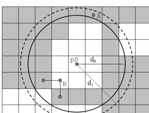
Here, we propose an alternative closed contour criteria that is largely insensitive to model resolution, using graph search to ensure that all paths along the unstructured grid from an initial locationp0 lead to a sufficiently large de-crease (or inde-crease) in a given field G before reaching a specified radius. This criteria is illustrated in Fig. 4, and is implemented in Algorithms 4 and 5 (for closed contours around local maxima). The closed contour criteria is im-plemented in TempestExtremes via the command line argu-ment - -closedcontourcmd. An analogous command line argument, - -noclosedcontourcmd, is also pro-vided, which has similar functionality but discards candi-dates that satisfy the closed contour criteria (this may be de-sirable, for instance, to identify cyclonic structures that do not have a warm core).

(5)

P. A. Ullrich and C. M. Zarzycki: A framework for scale-insensitive pointwise feature tracking₁₈ _{P. A. Ullrich and C. M. Zarzycki: A Framework for Scale-Insensitive Pointwise Feature Tracking} 1073

Algorithm 4Find the node pmaxcontaining the maximal value of the fieldGwithin a distancemaxdistof the node p. An analogous procedurefind_min_nearis provided for locating nodes containing minimal values of the field.

node pmax =

find_max_near(node p, field G, maxdist) set visited = {}

set tovisit = {p} pmax = p

while tovisit is not empty q = remove node from tovisit if (q in visited) then continue add q to visited

if (gcdist(p,q) > maxdist) then continue if (G[q] > G[pmax]) then pmax = q

Algorithm 5 Determine if there is a closed contour in fieldGof magnitudethresharound the pointp0, defined byp0 = find_max_near(p, G, maxdist), within distancedist. That is, along all paths away fromp0, the fieldGmust drop by at leastthreshwithin distancedist. The closed contour criteria is depicted in Fig. 54. An anal-ogous procedure is defined for closed contours around min-ima.

closed_contour_max(point p, field G, dist, maxdist, thresh)

p0 = find_max_near(p, G, maxdist) set visited = {}

set tovisit = {p0}

while tovisit is not empty q = remove point from tovisit if (q in visited) then continue add q to visited

if (gcdist(p0,q) > dist) then return false if (G[p0] - G[q] < thresh) then

add all neighbors of q to tovisit return true

Algorithm 6Determine if a candidate nodepsatisfies the requirement that there exists another nodep0within distance distofpwithG[p] > thresh.

threshold_max(node p, field G, dist, thresh)

p0 = find_max_near(p, G, dist) if (G[p0] < thresh) then

return false else

return true

Algorithm 7Determine all feature pathsS, given array of candidate nodes P[1..T] and maximum great-circle dis-tance between nodes at subsequent time levelsdist.

path set S = stitch_nodes(set array P[1..T], dist, maxgap)

for each time level t = 1..T K[t] = build_kd_tree(P[t]) for each time level t = 1..T

while P[t] is not empty initialize empty path s

p = remove next candidate from P[t] add p into s

gap = 0

for time level u = t+1..T

q = kd_tree_nearest_neighbor(K[u], p) if (q in P[u]) and (gcdist(p,q) < dist)

then add q into s remove q from P[u] p = q

else if (gap < maxgap) then gap = gap + 1

else break add s into S

Figure 51.An example node graph describing an unstructured grid (blue lines), where nodes are co-located with volume centerpoint locations (solid circles) and edges connect adjacent volumes.

Geosci. Model Dev., 10, 1–21, 2017 www.geosci-model-dev.net/10/1/2017/

18 P. A. Ullrich and C. M. Zarzycki: A Framework for Scale-Insensitive Pointwise Feature Tracking Algorithm 4Find the nodepmaxcontaining the maximal

value of the fieldGwithin a distancemaxdistof the node p. An analogous procedurefind_min_nearis provided for locating nodes containing minimal values of the field.

node pmax =

Algorithm 5 Determine if there is a closed contour in fieldGof magnitudethresharound the pointp0, defined byp0 = find_max_near(p, G, maxdist), within distancedist. That is, along all paths away fromp0, the fieldGmust drop by at leastthreshwithin distancedist. The closed contour criteria is depicted in Fig. 4. An anal-ogous procedure is defined for closed contours around min-ima.

set tovisit = {p0}

Algorithm 6Determine if a candidate nodepsatisfies the requirement that there exists another nodep0within distance distofpwithG[p] > thresh.

return false else

return true

Algorithm 7Determine all feature pathsS, given array of candidate nodes P[1..T] and maximum great-circle dis-tance between nodes at subsequent time levelsdist.

gap = 0

2.7 Thresholding

Additional threshold criteria may be applied at the detection stage in order to further eliminate undesirable candidates. For example, a common threshold criteria requires that a field G satisfy some minimum value within a distancedistof the candidate, as implemented in Algorithm 6. TempestEx-tremes implements thresholding via the command line argu-ment- -thresholdcmdand includes thresholds for a par-ticular field at candidate nodes to be greater than, less than, equal to or not equal to a specified value.

18 P. A. Ullrich and C. M. Zarzycki: A Framework for Scale-Insensitive Pointwise Feature Tracking

Algorithm 4 Find the node pmaxcontaining the maximal value of the fieldGwithin a distancemaxdistof the node p. An analogous procedurefind_min_nearis provided for locating nodes containing minimal values of the field.

node pmax =

Algorithm 5 Determine if there is a closed contour in fieldGof magnitudethresharound the pointp0, defined byp0 = find_max_near(p, G, maxdist), within distance dist. That is, along all paths away fromp0, the fieldGmust drop by at leastthreshwithin distancedist. The closed contour criteria is depicted in Fig. 54. An anal-ogous procedure is defined for closed contours around min-ima.

set tovisit = {p0}

Algorithm 6 Determine if a candidate nodepsatisfies the requirement that there exists another nodep0within distance distofpwithG[p] > thresh.

return false else

return true

Algorithm 7Determine all feature paths S, given array of candidate nodes P[1..T] and maximum great-circle dis-tance between nodes at subsequent time levelsdist.

gap = 0

2.8 Stitching

The basic track stitching procedure (which represents the Re-duce() stage in MapReduce) is implemented in Algorithm 7 using the output from the detection procedure at each time level (stored in set arrayP[1..T]). It requires additional parameters to specify a maximum great-circle distance be-tween in-sequence nodes (dist), and a maximum gap size (maxgap). Here, gap size refers to the maximum number of sequential non-detections that can occur before a path is considered terminated. This argument is useful, for instance, for tracking tropical storms that temporarily weaken below acceptable criteria before restrengthening.

18 P. A. Ullrich and C. M. Zarzycki: A Framework for Scale-Insensitive Pointwise Feature Tracking Algorithm 4Find the nodepmaxcontaining the maximal

value of the fieldGwithin a distancemaxdistof the node p. An analogous procedurefind_min_nearis provided for locating nodes containing minimal values of the field.

node pmax =

Algorithm 5 Determine if there is a closed contour in fieldGof magnitudethresharound the pointp0, defined byp0 = find_max_near(p, G, maxdist), within distancedist. That is, along all paths away from p0, the fieldGmust drop by at leastthreshwithin distancedist. The closed contour criteria is depicted in Fig. 54. An anal-ogous procedure is defined for closed contours around min-ima.

set tovisit = {p0}

Algorithm 6Determine if a candidate node psatisfies the requirement that there exists another nodep0within distance distofpwithG[p] > thresh.

return false else

return true

Algorithm 7Determine all feature pathsS, given array of candidate nodes P_[1..T_] and maximum great-circle dis-tance between nodes at subsequent time levelsdist.

gap = 0

For simplicity,k-d trees are constructed at each time level in order to maximize the efficiency of the search. Each can-didate pair (time, node) can only be used in one path, and so construction simply requires exhausting the list of available

(6)

Figure 3.An example two-dimensionalk-d tree (k=2) built from nodes a through h. Dividing planes are constructed by cycling through each coordinate and determining the median node (left). This gives rise to a tree structure (right) that, in conjunction with an input node, can then be searched recursively for a corresponding rectangular domain in physical space. The last leaf node is labeled as the best candidate for nearest neighbor and the tree is “unwound” to test other potential candidates. The number of nodes that need to be examined is limited to domains that overlap a hypersphere with origin at the input node and with distance to the current candidate.

Figure 4. An illustration of the closed contour criteria. Nodes shaded in white (gray) satisfy (do not satisfy) the threshold of the field value atp0. Since only edge neighbors are included,B con-stitutes a boundary to the interior of the closed contour. BecauseA lays outside the solid circle, the contour with distanced₀is not a closed contour, whereas the dashed contour with distanced₁does satisfy the closed contour criteria.

candidates. Once paths have been constructed, additional cri-teria can be applied – for instance, minimum path length or additional criteria based on minimum path length or mini-mum distance between the start and endpoints of the path (see Appendix E). Thresholds based on field values may also be applied; e.g., wind speed must be greater than a particular value for at least eight time steps of each track.

2.9 Parallelization considerations

Feature tracking fits well into a general framework known as MapReduce (Dean and Ghemawat, 2008), which is a combi-nation of a Map(), an embarrassingly parallel candidate iden-tification procedure applied to individual time slices, and a Reduce(), which stitches candidates across time to build fea-ture tracks. A key advantage of employing this framework is that substantial work has been undertaken to understand optimal strategies for parallelization of MapReduce-type al-gorithms (e.g., Prabhat et al., 2012) in order to mitigate bot-tlenecks associated with I/O and load balancing. TempestEx-tremes currently implements a simple parallelization strategy via MPI, although future work on this issue is forthcoming. As a timing example, TempestExtremes with MPI (16 tasks) finds and tracks tropical cyclones in 10 years of 6-hourly cli-mate data on a 0.5◦_{latitude–longitude grid in an average of}

3.8 min on the National Center for Atmospheric Research’s (NCAR’s) Yellowstone supercomputer.

3 Selected examples

Several selected examples are now provided. The first three examples use data from the NCEP Climate Forecast System Reanalysis (CFSR), available at 0.5◦_{global resolution with}

(7)

3.1 Tropical cyclones in CFSR

Our first example employs TempestExtremes for tropical cy-clones (defined here as a cyclonic structure with a distinct warm core). The command line we use to detect tropical cyclone-like features in CFSR is provided below. Climate data are drawn from three files denoted$uvfile (contain-ing zonal and meridional velocities),$tpfile(containing temperature and pressure information) and $hfile (con-taining topographic height). Three-dimensional (time plus 2-D space) hyperslabs of CFSR data have been extracted, with TMP_L100 corresponding to 400 hPa air tempera-ture, and U_GRD_L100and V_GRD_L100corresponding to 850 hPa zonal and meridional wind velocities. Candidates are initially identified by minima in the sea level pressure (PRMSL_L101), and then eliminated if a more intense mini-mum exists within a great-circle distance of 2.0◦_{. The closed}

contour criteria is then applied, requiring an increase in SLP of at least 200 Pa (2 hPa) within 4◦_{of the candidate node, and}

a decrease in 400 hPa air temperature of 0.4 K within 8◦_of

the node within 1.1◦_{of the candidate with maximum air}

tem-perature. Since CFSR is on a structured latitude–longitude grid, the output format isi,j,lon,lat,psl,maxu,zs, wherei,jare the longitude and latitude coordinates within the dataset;lon,latare the actual longitude and latitude of the candidate;pslis the SLP at the candidate point (equal to the maximum SLP within 0◦ _{of the candidate);}_maxu_is

the vector magnitude of the maximum 850 hPa wind within 4◦_{of the candidate; and}_zs_{is the topographic height at the}

candidate point.

./DetectCyclonesUnstructured

--in_data "$uvfile;$tpfile;$hfile" --out $outf

--searchbymin PRMSL_L101 --mergedist 2.0 --closedcontourcmd "PRMSL_L101,200.,4,0;

TMP_L100,-0.4,8.0,1.1" --outputcmd "PRMSL_L101,max,0;

_VECMAG(U_GRD_L100,V_GRD_L100),max,4; HGT_L1,max,0"

All outputs from DetectCyclonesUnstructured are then concatenated into a single file containing candidates at all times (pgbhnl.dcu_tc_all.dat). Candidates are then stitched in time to form paths, with a maximum distance be-tween candidates of 8.0◦_{(great-circle distance), consisting of}

at least eight candidates per path, and with a maximum gap size of two (most consecutive time steps with no associated candidate). Because localized shallow low-pressure regions that are unrelated to tropical cyclones can form as a con-sequence of topographic forcing, we also require that for at least eight time steps the underlying topographic height (zs) be at most 100 m. The associated command line for StitchN-odes is

./StitchNodes

--in pgbhnl.dcu_tc_all.dat --out pgbhnl.dcu_tc_stitch.dat --format "i,j,lon,lat,psl,maxu,zs"

Figure 5.Tropical cyclone counts within each 2◦×2◦grid cell, over the period 1979–2010, obtained using the procedure described in Sect. 3.1.

--range 8.0 --minlength 8 --maxgap 2 --threshold "zs,<=,100.0,8"

Once the complete set of tropical cyclone paths has been computed, total tropical cyclone counts over each 2◦_{grid cell}

are plotted in Fig. 5. The results show very good agreement with reference fields (Gray, 1968; Knapp et al., 2010). 3.2 Extratropical cyclones in CFSR

For our second example, we are interested in tracking ex-tratropical cyclone features (defined by a cyclonic structure with no distinct warm core). The command line we have used to detect cyclonic features without the characteristic warm core of tropical cyclones (here referred to as extrat-ropical cyclones) is given below. The command is identical to the tropical cyclone (TC) detection configuration speci-fied in Sect. 3.1, except it requires that the feature does not possess a closed contour in the 400 hPa temperature field (no warm core).

--in_data "$uvfile;$tpfile;$hfile" --out $outf

--searchbymin PRMSL_L101 --mergedist 2.0 --closedcontourcmd "PRMSL_L101,200.,4,0" --noclosedcontourcmd "TMP_L100,

-0.4,8.0,1.1"

--outputcmd "PRMSL_L101,max,0;

_VECMAG(U_GRD_L100,V_GRD_L100),max,4; HGT_L1,max,0"

Stitching is similarly analogous to Sect. 3.1, except it uses a slightly more strict criteria on the underlying topographic height. The topographic filtering proved necessary in order to adequately filter out an abundance of topographically driven low pressure systems, particularly in the Himalayas region. The command line used for stitching is given below:

./StitchNodes

--in pgbhnl.dcu_tc_all.dat

(8)

Figure 6.Extratropical cyclone counts within each 2◦×2◦grid cell, over the period 1979–2010, obtained using the procedure described in Sect. 3.2.

--out pgbhnl.dcu_tc_stitch.dat --format "i,j,lon,lat,psl,maxu,zs" --range 8.0 --minlength 8 --maxgap 2 --threshold "zs,<=,70.0,8"

Once the complete set of extratropical cyclone paths has been computed, total extratropical cyclone density over each 2◦_{grid cell is plotted in Fig. 6. Although not extensively}

ver-ified, the qualitative density of extratropical cyclones is well within the range of results from different trackers, as given by Neu et al. (2013).

3.3 Tropical easterly waves in CFSR

Tropical easterly waves are our third example of a pointwise feature that has been assessed in the track-ing literature. In this example, Northern Hemisphere east-erly waves (associated with positive relative vorticity) are tracked separately from Southern Hemisphere east-erly waves (associated with negative relative vorticity). DetectCyclonesUnstructured andStitchNodes are executed separately in both hemispheres and the re-sultant track files concatenated. All tracking is performed on the 600 hPa relative vorticity field, using relative vor-ticity maxima for Northern Hemisphere waves and rel-ative vorticity minima for Southern Hemisphere waves. Since CFSR only provides absolute vorticity, relative vor-ticity must first be extracted by taking the difference be-tween absolute vorticity and the planetary vorticity (the Coriolis parameter). This is done on the command line via _DIFF(ABS_V_L100,_F()), where ABS_V_L100 is the CFSR absolute vorticity variable and_F()is a built-in function for computbuilt-ing the Coriolis parameter (defbuilt-ined by f =2sinφ). In the Northern Hemisphere, we follow Thorncroft and Hodges (2001) and isolate tropical easterly wave features by requiring a drop of relative vorticity equal to 5×10−5_s−1_{. The command line used is as follows:}

--in_data "$uvfile;$hfile" --out $outf

--searchbymax "_DIFF(ABS_V_L100(0),_F())" --mergedist 2.0

--closedcontourcmd "_DIFF(ABS_V_L100(0), _F()),-5.e-5,4,0"

--outputcmd "ABS_V_L100(0),max,0 ;_DIFF(ABS_V_L100(0),_F()),max,0;

HGT_L1,max,0"

--minlat -35.0 --maxlat 35.0

Tropical easterly wave paths are constructed using a maxi-mum distance of 3◦_{great-circle distance between subsequent}

detections, a minimum path length equal to eight sequential detections, no allowed gaps, and a distance of at least 10◦

between track start and endpoint. Northern (Southern) Hemi-sphere waves must also be present in the Northern (Southern) Hemisphere for at least eight time steps (2 days). The com-mand line for Northern Hemisphere waves is as follows:

./StitchNodes

--in pgbhnl.dcu_aew_nh_all.dat --out pgbhnl.dcu_aew_nh_stitch.dat --format "i,j,lon,lat,relv,zs" --range 3.0 --minlength 8 --maxgap 0 --min_endpoint_dist 10.0

--threshold "lat,<=,25.0,8;lat,>=,0.0,8" An analogous procedure is applied in the Southern Hemi-sphere, except it searches for minima in the relative vorticity field and limits the latitudinal range inStitchNodesto [25S,0] for at least eight time steps. Counts of total (North-ern Hemisphere plus South(North-ern Hemisphere) tropical easterly waves within each 2◦_{grid volume are given in Fig. 7,}

show-ing heavy wave activity throughout the Atlantic and Pacific basins. These results are very similar to other reported east-erly wave densities, such as in Belanger et al. (2014) and Thorncroft and Hodges (2001), except for (a) the substan-tially enhanced tropical easterly wave count reported over eastern Africa (which could be eliminated by filtering over topography) and (b) essentially no observed wave activity off of the western coast of South America. Nonetheless, it is well known that easterly wave climatology varies strongly across reanalysis datasets and exhibits sensitivity to the choice of tracking scheme (Hodges et al., 2003).

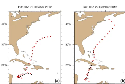
3.4 Tropical cyclone forecast trajectories

For our third example, we have used TempestExtremes to track forecasted tropical cyclones in numerical weather pre-diction simulations. Here, we show two deterministic fore-casts (initialized at 00Z on 21 and 22 October 2012) for Hurricane Sandy using the Community Atmosphere Model (CAM) with a 0.125◦ _{(14 km) grid spacing over the North}

(9)

Figure 7.Tropical easterly wave counts within each 2◦×2◦grid cell, over the period 1979–2010, obtained using the procedure de-scribed in Sect. 3.3.

Figure 8.Forecast CAM trajectories for Hurricane Sandy initial-ized at 00Z on(a)21 and(b)22 October 2012. Black dots indicate trajectories defined using the NCEP operational vortex tracker with red dots denoting trajectories defined using a sample configuration of TempestExtremes.

Prediction (NCEP) (Marchok, 2002) while red dots show the same using a sample configuration of TempestExtremes. This configuration finds local minima in the 6-hourly SLP (slp) fields, which cannot lie within a great-circle distance of 10.0◦

of another. An increase in SLP of at least 0.5 hPa within 5◦

of the candidate node is required (closed contour) as is a de-crease in 300 hPa air temperature (tm) of 0.1 K within 5◦_of

the node, with a 1.0◦_{offset permitted between the upper-level}

warm core maximum and sea level pressure minimum (rele-vant for sheared TCs where the vortex may be tilted). Note that no “best guess initial location” of the cyclone is defined, as is the case with many operational tracking systems. The tracker command line is as follows:

./DetectCyclonesUnstructured --in_data $ffile --out $outf

--mergedist 10.0

--closedcontourcmd "slp,0.5,5.0,0;tm,

Figure 9.An illustration of how connectivity is defined in this work for nodes on a spectral element mesh. Arrows indicate connectivity for nodes A and B.

-0.1,5.0,1.0"

--outputcmd slp,min,0;_VECMAG(u850,v850), max,2;_VECMAG(u_ref,v_ref),max,2"

./StitchNodes --in cand.cyc --out forecast.traj

--format "i,j,lon,lat,slp,wind850,windbot" --range 6.0 --minlength 8 --maxgap 2

The results here demonstrate good agreement with the NCEP vortex tracker, highlighting the capability of this framework to track even pre-genesis storm features, although the sensitivity (and associated potential noise) required to find weak, shallow or sheared storms depends on the thresh-olds defined in DetectCyclonesUnstructured. Some differences between tracked storm centers are noted, particularly at the beginning of the forecasts, where the storm’s SLP is greater (weaker) than 1005 hPa. This is due to the fact that the pre-genesis vortex is naturally somewhat disorganized, and the NCEP tracker uses an average of mul-tiple primary fixes (e.g., 700 and 850 hPa relative vorticity, sea level pressure, 700 and 850 hPa geopotential heights) to define the cyclone center, whereas this configuration of TempestExtremes defines storm location based on sea level pressure minimum only.

3.5 Tropical cyclones in a simulation with VR-CAM

For our final example, we assess the differences in tropical cyclone character obtained from native and regridded datasets. Using the variable-resolution spectral element option in CAM (VR-CAM-SE; Neale et al., 2012; Zarzycki et al., 2014b) to refine the Northern Hemisphere to 0.25◦ _{resolution, a simulation of}

a hurricane season (June–November) has been performed. With the high-order spectral element dynamical core used to solve the fluid equations in the atmosphere, VR-CAM-SE has been demonstrated to be effective in simulating tropical cyclone-like features (Zarzycki and Jablonowski, 2014;

(10)

Figure 10.Tropical cyclone trajectories and associated intensities as obtained from the simulation of a single hurricane season in CAM 3.5 using (top) native spectral element grid data and (bottom) data regridded to a regular latitude–longitude grid with 0.25◦_{grid spacing.}

Zarzycki et al., 2014a; Zarzycki and Jablonowski, 2015). Since VR-CAM-SE uses an unstructured mesh with degrees of freedom stored at spectral element Gauss–Lobatto (GL) nodes, data are typically analyzed only after being regridded to a regular latitude–longitude mesh of approximately equal resolution. The regridding procedure has the potential to clip local extrema and smear out grid-scale features.

For this example, we use the high-order regridding pack-age TempestRemap (Ullrich and Taylor, 2015; Ullrich et al., 2016) for remapping the native spectral element output to a regular latitude–longitude grid with 0.25◦ _{grid spacing.}

For purposes of determining connectivity on the variable-resolution spectral element mesh, we connect GL nodes along the coordinate axis of each quadrilateral element (see Fig. 9). DetectCyclonesUnstructured is then applied to both the native grid data and the regridded data on the regular latitude–longitude mesh (using the configuration specified in Sect. 3.1) and tropical cyclones are categorized (color-coded) by maximum surface wind speed as defined by the Saffir– Simpson scale (Simpson, 1974), such that orange and red trajectories represent the strongest classifications of storms. The results of this analysis are depicted in Fig. 10. As ex-pected, the native grid output produces essentially identical tracks, but an increase in tropical cyclone intensity in some cases (with some tropical cyclones dropping down by a full category as a consequence of the remapping procedure and discrete nature of binning storm strength).

4 Conclusions

Automated pointwise feature trackers have been frequently and successfully employed over the past several decades to extract useful information from large climate datasets. With spatial and temporal resolution increasing rapidly in response to enhanced computational resources, climate datasets have grown increasingly unwieldy and so there has been a grow-ing need for such large dataset processgrow-ing tools. This pa-per has outlined a framework for pointwise feature tracking (TempestExtremes) that exposes a suite of generalized ker-nels drawn from the literature on trackers of the past several decades. This framework is sufficiently robust to be appli-cable to many climate and weather datasets, including data on unstructured grids. We expect such a framework would be useful for isolating uncertainties that emerge from partic-ular parameter choices in tracking schemes, or to compute optimal threshold values for detecting pointwise features in, e.g., reanalysis data. Future development plans in Tempes-tExtremes include the construction of analogous kernels for tracking areal features (blobs), such as clouds or atmospheric rivers.

5 Code availability

(11)

Appendix A: A review of extratropical cyclone tracking algorithms

This appendix reviews the existing literature on extratropical cyclone tracking, one of the earliest and most common in-stances of both manual and automated feature tracking. Man-ual counts of cyclones were performed by Petterssen (1956) in the Northern Hemisphere from 1899 to 1939, and latter binned by Klein (1957) to determine the spatial distribution of such storms. These techniques were later refined by Whit-taker and Horn (1982) by accounting for cyclone trajecto-ries. A similar survey in the Southern Hemisphere was per-formed by Taljaard (1967) for July 1957–December 1958. Manual tracking and characterization of cyclones was also performed by Akyildiz (1985) using ECMWF forecast data for the 1981/1982 winter.

One of the first automated detection and tracking for ex-tratropical cyclones was developed by Williamson (1981) us-ing nonlinear optimization to fit cyclonic profiles to anoma-lies in the 500 mb geopotential height field. Storms were then tracked over a short forecast period using the best fit to the cyclone’s center point. Counts of cyclones neglecting the cy-clone trajectory were automatically generated from climate model output for both hemispheres by Lambert (1988) using local minima in 1000 hPa geopotential height. This method had some shortcomings, including mischaracterization of lo-cal lows due to Gibbs’ ringing and topographilo-cally driven lows. To overcome these problems, Alpert et al. (1990) pro-posed an additional minimum threshold on the local pressure gradient. Similarly, Le Treut and Kalnay (1990) detected cy-clones in ECMWF pressure data using a local minima in the sea level pressure that must also be 4 hPa below the aver-age sea level pressure of neighboring grid points, and must persist for three successive 6 or 12 h intervals. Murray and Simmonds (1991) extracted low pressure centers from inter-polated general circulation model (GCM) data using local optimization, based on earlier work in Rice (1982). These original papers primarily sought minima in the SLP field or looked for maxima in the Laplacian of the SLP field.

Several modern extratropical cyclone detection algorithms remain in use, having built on this earlier work. Short de-scriptions of many of these schemes are given here. Some of these algorithms use the notion of a local neighborhood or periphery, as defined in Fig. A1.

– Serreze et al. (1993); Serreze (1995) tracked cyclones in a ∼381–400 km Arctic dataset. Candidates were identified using a local minimum SLP at least 2 hPa higher than immediate neighbors. Tracking was per-formed with a maximum search distance of 1400 km per 12 h period.

– Sinclair (1994, 1997) tracked cyclones in a 2.5◦

ECMWF dataset over the Southern Hemisphere. Can-didates were identified using a local minimum in the 1000 hPa geostrophic vorticity fieldζ_g(computed from

Figure A1.The local neighborhood of a central node (shaded) typi-cally refers to the surrounding eight nodes (diagonal hatching). The periphery, used by Tsutsui and Kasahara (1996), refers to the set of nodes that surround the local neighborhood (unshaded nodes).

the Laplacian of the 1000 hPa geopotential), adjusted for topography and the presence of heat lows (see paper for details), which further satisfiedζ_g<−2×10−5s−1. – Blender et al. (1997) tracked cyclones in T106 (∼125 km) ECMWF analyses. Candidates were iden-tified using a local minimum in the 1000 hPa geopoten-tial height field, and required to have a positive mean gradient in the 1000 hPa geopotential height field in a 1000×1000 km2_{area around each candidate. Tracking} was performed using a nearest-neighbor search with a maximum displacement velocity of 80 km h−1_, elimi-nating cyclones with tracks shorter than 3 days. – Lionello et al. (2002) tracked cyclones in a T106

(∼125 km) ECHAM-4 dataset. Candidates were iden-tified using a local minimum in the SLP field. Track-ing was performed usTrack-ing previous cyclone velocity to demarcate a prediction region, and candidates were dis-carded if they do not continue into the prediction region. – Zolina and Gulev (2002) tracked cyclones in a T106 (∼125 km) and a T42 (∼300 km) dataset. Candidates were identified using a local minimum in the SLP field. – Hoskins and Hodges (2002); Catto et al. (2009); Dacre et al. (2012) tracked cyclones in various reanalysis and climate datasets with wavenumber≤5 removed in all fields and a relative vorticity field spectrally truncated to T42. Candidates were identified from maxima in the

(12)

850 hPa relative vorticity field. Trajectories were com-puted by searching for nearest neighbors and smoothed by minimizing a cost function. Cyclones were required to persist for 4 days.

– Pinto et al. (2005) tracked cyclones in T42 (∼300 km) NCEP reanalysis, regridded onto a 0.75◦ _{grid by}

cu-bic spline interpolation. Candidates were identified us-ing local minima in the pressure field that were within 1200 km of a maximum in the quasi-geostrophic rela-tive vorticity, which was computed from the Laplacian of pressure. Candidates that were over a topography of above 1500 m were removed. They further required that the quasi-geostrophic relative vorticity was greater than 0.1 hPa/ (◦lat)and only the strongest candidates within 3◦_{were retained. Cyclone tracking required a prediction}

velocity and search following Murray and Simmonds (1991).

– Benestad and Chen (2006) tracked cyclones in 2.5◦

ERA40 data. Candidates were identified using multiple least-squares regression to estimate the values of the co-efficients of a Fourier approximation to the SLP field (in effect a smoothing operator), followed by a 1-D search in the north–south and east–west directions.

– Simmonds et al. (2008) tracked cyclones in several 2.5◦

datasets over the Arctic. Candidates were identified us-ing local minima in the Laplacian of pressure, reject-ing cyclones over topography above 1000 m and re-quiring the presence of a nearby pressure minimum. Identified lows must satisfy a Laplacian with value> 0.2 hPa/ (◦lat)2 over a radius of 2◦. Tracking used a probability estimate using a predicted position.

Appendix B: A review of tropical cyclone tracking algorithms

More recently, and as higher-resolution climate data have become available, extratropical cyclone tracking techniques have been modified in order to support tropical cyclone tracking. To eliminate “false positives” associated with ex-tratropical cyclones and weak cyclonic depressions, many schemes require that the candidate be associated with a nearby warm core and be associated with a minimum thresh-old on surface winds for at least 1–3 days. The definition of a “warm core” varies between modeling centers, includ-ing such options as air temperature anomaly on pressure surfaces (Vitart et al., 1997; Zhao et al., 2009; Murakami et al., 2012), geopotential thickness (Tsutsui and Kasahara, 1996) and decay of vorticity with height (Bengtsson et al., 2007a; Strachan et al., 2013). Additional filtering of candi-date storms over topography or within a specified latitudi-nal range may be required. To better match observations, ad-ditional geographical-, model- or feature-dependent criteria

may be applied (Camargo and Zebiak, 2002; Walsh et al., 2007; Murakami and Sugi, 2010a; Murakami et al., 2012). It is widely acknowledged that weaker tropical storms are difficult to track, and the observational record of these less-intense, short-lived storms is questionable (Landsea et al., 2010).

A tabulated overview of the thresholds utilized by many of these schemes can be found in Walsh et al. (2007), along with several proposed guidelines on detection schemes. We extend this tabulation with the following short descriptions of many published schemes.

– Bengtsson et al. (1982) tracked tropical cyclones in one year of ∼200 km forecast model output. Candi-dates were identified with latitude<30◦for collocated 850 hPa wind>25 m s−1and 850 hPa relative vorticity maxima>7×10−5s−1in a 7.5◦×7.5◦area.

– Broccoli and Manabe (1990) tracked tropical cyclones in a R15 (∼600 km) dataset and a R30 (∼300 km) dataset. Candidates were identified from PSL that had a 1.5 hPa local min (R15) or 0.75 hPa local min (R30), with local surface wind velocity > 17 m s−1, and latitude < 30◦. Tracking was performed using nearest-neighbor search with a maximum velocity of 1200 km day−1_.

– Wu and Lau (1992) tracked tropical cyclones in a 7.5◦longitude×4.5◦latitude dataset. Candidates were identified by local minima in 1000 hPa geopotential height with a positive 950 hPa relative vorticity, negative 950 hPa divergence, positive 500 hPa vertical velocity, latitude<40.5◦, locally maximal 200 h minus 1000 hPa layer thickness that exceeded the average layer thick-ness within 1500 km west to east by 60 m, and 950 hPa wind greater than 17.2 m s−1_{locally. Tracking imposed} a maximum tropical cyclone velocity of 7.5◦_longitude

or 9◦_{latitude per day.}

– Haarsma et al. (1993) tracked tropical cyclones in a

∼300 km dataset. Candidates were identified from lo-cal minimum PSL, with 850 hPa relative vorticity > 3.5×10−5s−1. Temperature anomaly1T was required to satisfy1T250>0.5 K at 250 hPa,1T500>−0.5 K at 500 hPa, and1T250−1T850>−1.0 K, where the anomaly is computed against a 15◦_×₁₅◦_{spatial mean}

around the center of the storm. Tracking required tropi-cal cyclones to be persistent for a minimum of 3 days. – Bengtsson et al. (1995, 1996) tracked tropical cyclones

(13)

1T300> 1T850 where the anomaly was computed against a 7×7 grid-point average centered on the can-didate. Tracking required tropical cyclones to be persis-tent for a minimum of 1.5 days.

– Tsutsui and Kasahara (1996) tracked tropical cyclones in a T42 (2.8◦_, _∼_{300 km) dataset. Candidates were}

identified as minima in the 1000 hPa geopotential height field, with at least an average drop of 20 m among neigh-boring points, and a further 20 m drop of average among neighboring points from periphery. Candidates were further required to satisfy that the average local 900 hPa vorticity was cyclonic, average local 900 hPa divergence was negative, average local 500 hPa vertical velocity was upward, 200 hPa minus 1000 hPa layer thickness maximum among neighbors was greater than any value in periphery, and average local 200 hPa zonal wind ve-locity was less than 10 m s−1_{or local points contained} at least one point with easterly velocity. The latitude of the candidate was require to be less than 40◦_,

topo-graphic height underlying candidates was less than 400 m, one local point had a 900 hPa wind speed of at least 17.2 m s−1_{, and one local point exceeded 100 mm d}−1 over at least 1 day. Tracking required tropical cyclones to be persistent for a minimum of 2 days.

– Vitart et al. (1997, 1999, 2001, 2003) tracked tropical cyclones in a T42 (2.8◦_,_∼_{300 km) dataset. Candidates}

were identified as 850 hPa relative vorticity maxima >3.5×10−5s−1 with a nearby PSL minimum. They were required to possess a warm core within 2◦_latitude,

defined as a local average 500 hPa to 200 hPa tempera-ture maximum with a decrease of 0.5 K in all directions within 8◦_{, and a local maximum in the 200–1000 hPa}

layer thickness with a decrease of 50 m in all directions within 8◦_{. Tracking required the minimum distance}

be-tween storms to be 800 km day−1_{, that tropical cyclones} lasted at least 2 days and that the maximum wind veloc-ity within 8◦_{of the storm center must be 17 m s}−1_{for at} least 2 (not necessarily consecutive) days.

– Walsh (1997); Walsh and Watterson (1997); Walsh and Katzfey (2000) tracked tropical cyclones in a 125 km re-gional climate dataset over Australia. Candidates were identified as points with 850 hPa relative vorticity > 2.0×10−5_s−1_{, temperature anomaly sum} _1T₇₀₀₊ 1T500+1T300>0 K and 1T300> 1T850, with anomaly computed against the mean over a region 2 grid points north–south and 13 grid points east–west. Candidates were also required to have 10 m surface wind >10 m s−1 and 850 hPa tangential wind speed >300 hPa tangential wind speed. Tracking required tropical cyclones to be persistent for a minimum of 2 days.

– Krishnamurti et al. (1998) tracked tropical cyclones in a T42 (∼300 km) climate dataset. Their approach was

similar to Bengtsson et al. (1995, 1996), except using a 4×4 grid-point region for the 850 hPa wind maximum, the SLP minimum and the temperature mean. Tracking required tropical cyclones to be persistent for a mini-mum of 1 day.

– Nguyen and Walsh (2001) assessed a 125 km regional dataset over Australia using a similar approach to Walsh and Watterson (1997). The vorticity requirement was changed to 850 hPa relative vorticity>1.0×10−5s−1 with a PSL minimum within 250 km. Candidates also must possess a mean wind speed in a 500 km×500 km region at 850 hPa that was larger than mean wind speed at 300 hPa, and a mean tangental wind speed within a radius of 1◦_{and 2.5}◦_{greater than 5 m s}−1_{. Tracking} re-quired tropical cyclones to be persistent for a minimum of 1 day, with relaxed criteria after this time (see paper for further information).

– Sugi et al. (2002) tracked tropical cyclones in a T106 (∼125 km) climate dataset, using tracking criteria sim-ilar to Bengtsson et al. (1995). Candidates were identi-fied by local PSL minima that was at least<1020 hPa. Tracking required tropical cyclones to be persistent for a minimum of 2 days.

– Camargo and Zebiak (2002) tracked tropical cyclones in a T42 (∼300 km) climate dataset. Their approach was similar to Bengtsson et al. (1995, 1996), except with basin-specific thresholds are applied for 850 hPa relative vorticity, 850 hPa wind speed, and temperature anomaly sum1T700+1T500+1T300. Thresholds were determined by sampling the tails of probability density functions for relevant variables in each ocean basin. Following candidate identification, a relaxed 850 hPa relative vorticity threshold (>1.5×10−5_s−1₎ in an area of 3×3 grid points around prior detections was applied to construct trajectories. Tracking required tropical cyclones to be persistent for a minimum of 2 (1.5) days in daily (6-hourly) output.

– Tsutsui (2002) tracked tropical cyclones in a T42 (2.8◦_,

∼300 km) dataset. Their approach was similar to Tsut-sui and Kasahara (1996), but with simplified criteria. Candidate PSL was required to be less than the lo-cal average minus 2 hPa, and lolo-cal average PSL must be less than the periphery average minus 2 hPa. Layer thickness between 200 and 700 hPa, denoted byZ, was required to satisfy Z₀+max(Z_±₁1) >2max(Z_±21),

whereZ_±11 denotes immediate neighbors and Z_±21

denotes the periphery.

– Cheung and Elsberry (2002); Halperin et al. (2013) tracked tropical cyclones in weather forecast models us-ing an approach similar to Walsh (1997). Candidates re-quired a grid-point maximum in 850 hPa relative vortic-ity larger than all surrounding grid points within 4◦_and