www.earth-syst-sci-data.net/9/63/2017/ doi:10.5194/essd-9-63-2017
© Author(s) 2017. CC Attribution 3.0 License.
A sudden stratospheric warming compendium
Amy H. Butler1,2, Jeremiah P. Sjoberg1,2, Dian J. Seidel3,*, and Karen H. Rosenlof2
1Cooperative Institute for Research in Environmental Sciences, University of Colorado, Boulder,
CO 80309, USA
2National Oceanic and Atmospheric Administration, Earth Systems Research Laboratory,
Chemical Sciences Division, Boulder, CO 80305, USA
3National Oceanic and Atmospheric Administration, Air Resources Laboratory, College Park, MD 20740, USA
*retired
Correspondence to:Amy H. Butler ([email protected])
Received: 23 September 2016 – Discussion started: 27 September 2016 Revised: 20 December 2016 – Accepted: 5 January 2017 – Published: 9 February 2017
Abstract. Major, sudden midwinter stratospheric warmings (SSWs) are large and rapid temperature increases in the winter polar stratosphere are associated with a complete reversal of the climatological westerly winds (i.e., the polar vortex). These extreme events can have substantial impacts on winter surface climate, including increased frequency of cold air outbreaks over North America and Eurasia and anomalous warming over Greenland and eastern Canada. Here we present a SSW Compendium (SSWC), a new database that documents the evolution of the stratosphere, troposphere, and surface conditions 60 days prior to and after SSWs for the period 1958–2014. The SSWC comprises data from six different reanalysis products: MERRA2 (1980–2014), JRA-55 (1958–2014), ERA-interim (1979–2014), ERA-40 (1958–2002), NOAA20CRv2c (1958–2011), and NCEP-NCAR I (1958– 2014). Global gridded daily anomaly fields, full fields, and derived products are provided for each SSW event. The compendium will allow users to examine the structure and evolution of individual SSWs, and the variability among events and among reanalysis products. The SSWC is archived and maintained by NOAA’s National Centers for Environmental Information (NCEI, doi:10.7289/V5NS0RWP).
1 Introduction
The winter polar stratosphere is highly dynamic. In the Northern Hemisphere (NH), breaking planetary-scale waves propagating up from the troposphere or the excitation of reso-nant modes can lead to the disruption and deceleration of the climatological westerly circulation of the polar vortex (see Schoeberl, 1978 for a historical review). Associated with this wind deceleration is a dramatic warming, sometimes increas-ing the temperature of the polar stratosphere by as much as 30–40 K in a few days. In the most extreme cases, the strato-spheric polar vortex can reverse direction completely in an event called a major sudden stratospheric warming (SSW). SSWs in the NH occur roughly six times per decade (Charl-ton and Polvani, 2007). SSWs can also occur in the Southern Hemisphere (SH), as in a remarkable case in September 2002
(Kruger et al., 2005), but are rare due to smaller planetary wave amplitudes in the SH (van Loon et al., 1973).
Large perturbations in the stratospheric circulation can drive changes in surface climate for days to weeks (Kidston et al., 2015). In particular, SSWs are often followed by an equatorward shift of the North Atlantic tropospheric storm track, projecting onto the spatial pattern of the negative phase of the North Atlantic Oscillation (NAO). On average, this pattern results in warm anomalies over Greenland, eastern Canada, and subtropical Africa and Asia and cold anomalies over northern Eurasia and the eastern United States. How-ever, the impacts of individual SSWs vary widely, depending on the evolution of the vortex breakdown, the strength of the stratospheric–tropospheric coupling, and the state of the tro-pospheric climate.
poten-tial influence on ozone and chemical transport (e.g., Man-ney et al., 2009; Schoeberl and Hartmann, 1991), tropical convection and dynamics (e.g., Gómez-Escolar et al., 2014; Kodera, 2006), and mesospheric processes (e.g., Hoffmann et al., 2007), a research-ready database of these events would be useful. Daily three-dimensional gridded variables are needed to examine the full evolution and impacts of SSWs. There-fore, reanalysis products, which assimilate observations to constrain a global climate model, are often used. However, the calculation of daily anomalies or additional derived prod-ucts using reanalysis data can be computationally expensive and storage intensive. In addition, different reanalyses also differ in time spans, assimilated observations, assimilation scheme, parameterizations, and model physics. This makes intercomparison of multiple reanalysis products useful for assessing what features of SSWs and their associated climate variability are robust.
Here we describe a SSW Compendium (SSWC), which provides a detailed historical dataset of major SSWs, allow-ing users to consider the development, evolution, and impacts of individual SSWs and to provide a basis for model evalua-tion and improvement. A compendium is a concise compila-tion of comprehensive informacompila-tion on a specific subject, and therefore is an appropriate term to describe this dataset. The SSWC includes data from six established reanalysis ucts and includes anomaly fields and additional derived prod-ucts to highlight the dynamics and effects of SSW events. We present an overview of the reanalysis source data and the methodology for SSW event selection and data process-ing in Sect. 2. Section 3 discusses potential applications of this database, and Sect. 4 highlights the availability of the database at the National Oceanic and Atmospheric Admin-istration (NOAA) National Centers for Environmental Infor-mation (NCEI) archives and at the NOAA Earth Systems Re-search Laboratory (ESRL).
2 Methodology
2.1 Reanalysis data
The SSWC comprises data from six different reanalyses (Ta-ble 1): the National Aeronautics and Space Administration (NASA) Modern-Era Retrospective-analysis for Research and Applications version 2 (MERRA2), Japanese 55-year Reanalysis (JRA-55), European Centre for Medium-Range Weather Forecasts (ECMWF) 40-year Reanalysis (ERA-40), ECMWF Interim Reanalysis (ERA-interim), NOAA 20th Century Reanalysis version 2c (NOAA20CRv2c), and NOAA’s National Centers for Environmental Predic-tion/National Center for Atmospheric Research (NCEP-NCAR I) reanalysis.
Reanalyses are derived from observations from multi-ple sources (including surface observations, aircraft, ra-diosondes, rocketsondes, and satellites) that are assimilated by global coupled land–atmosphere–ocean models to
cre-ate spatially and temporally complete observational records. There are advantages and disadvantages of using reanalysis products for this database, as opposed to individual measure-ment sources or various stratospheric analyses. These anal-yses include that from the Freie Universitat Berlin, which produces a database of continuous daily gridded synoptic-scale analyses based largely on radiosonde measurements, but only for three stratospheric levels for a 35-year period (Labitzke and Collaborators, 2002), and from the NOAA Cli-mate Prediction Center (CPC), which offers analyzed strato-spheric temperatures at eight stratostrato-spheric levels based on satellite retrievals of the advanced microwave sounding unit (AMSU). The major advantage of reanalysis is that it al-lows consideration of the evolution of SSWs and their im-pacts throughout the entire atmosphere with a spatial and temporal extent that is not feasible using individual measure-ments or stratospheric analyses alone. A major disadvantage of using reanalysis is that due to sparse observations, particu-larly in the pre-satellite era, stratospheric reanalysis is poorly constrained, especially above 10 hPa (Manney et al., 2003), and tropospheric reanalysis may be poorly constrained over oceans and remote regions (e.g., Bosilovich et al., 2008). Re-analyses can also suffer from upper-boundary effects and dis-continuities due to model streams or changes in the observa-tions being assimilated (Fujiwara et al., 2016; Labitzke and Kunze, 2005). These issues should not have a strong effect on the daily-to-seasonal timescales documented in the SSWC, but should be kept in mind, especially for data above 10 hPa where the discontinuities are conspicuous.
Some biases and uncertainties in individual reanalysis products have been documented (see references in Table 1), and an evaluation of their stratospheric processes is cur-rently the focus of an international effort by the Stratosphere-troposphere Processes And their Role in Climate (SPARC) Reanalysis Intercomparison Project (S-RIP; Fujiwara et al., 2016). While initial studies have shown that stratospheric dy-namics and variability of and coupling to the surface are rea-sonably simulated in reanalyses (Martineau and Son, 2010), particularly in the latest generation products (Martineau et al., 2016), the SSWC enables quick comparison between re-analyses of sudden stratospheric warming events and their evolution on daily timescales. This capability is important when considering the substantial volume of data needed to calculate the daily climatology and anomalies for each grid point and pressure level in each reanalysis.
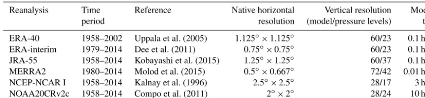
Table 1.The reanalyses included in the SSW Compendium.
Reanalysis Time Reference Native horizontal Vertical resolution Model
period resolution (model/pressure levels) top
ERA-40 1958–2002 Uppala et al. (2005) 1.125◦×1.125◦ 60/23 0.1 hPa ERA-interim 1979–2014 Dee et al. (2011) 0.75◦×0.75◦ 60/23 0.1 hPa JRA-55 1958–2014 Kobayashi et al. (2015) 1.25◦×1.25◦ 60/37 0.1 hPa MERRA2 1980–2014 Molod et al. (2015) 0.5◦×0.667◦ 72/42 0.01 hPa NCEP-NCAR I 1958–2014 Kalnay et al. (1996) 2.5◦×2.5◦ 28/17 3 hPa NOAA20CRv2c 1958–2014 Compo et al. (2011) 2◦×2◦ 28/24 10 hPa
ozone at high latitudes, leading to potentially high errors (De-thof and Hólm, 2004; Dragani, 2011).
In addition, the evolution of SSW events prior to 1964, when concentrated efforts to observe the upper atmosphere using radiosondes and rocketsondes were begun in associa-tion with the Internaassocia-tional Years of the Quiet Sun (IQSY), should be viewed with skepticism. Even radiosonde mea-surements of the stratosphere were very limited during that time period, and so reanalysis fields may be almost entirely model-driven.
The NOAA20CRv2c is unique among the reanalyses, be-cause it assimilates only surface pressure observations. Thus, the stratosphere is not constrained by any stratospheric obser-vations, and the reanalysis winds are not realistic (Compo et al., 2011). However, because surface pressure observations do a reasonable job of constraining the model throughout the northern hemispheric troposphere (Compo et al., 2011), we include the NOAA20CRv2c to examine the tropospheric im-pacts of SSWs, using SSW event dates given by the JRA-55 reanalysis (Table 2). The NOAA20CRv2c reanalysis pro-vides the unique opportunity to examine tropospheric and stratospheric interaction prior to and following SSWs, when only the surface is constrained by observations.
2.2 Event selection
MajorSSWs occur when the winter polar stratospheric west-erlies reverse to eastwest-erlies. Inminor warmings, the polar tem-perature gradient reverses but the circulation does not, and in final warmings, the vortex breaks down and remains easterly until the following boreal autumn. Because no unambiguous standard definition for major, minor, and final warmings yet exists (Butler et al., 2015), selecting SSW events to include in the Compendium is not straightforward.
The primary goal of the SSWC is to provide data for major SSWs, which have been found to have the largest surface im-pacts (Palmeiro et al., 2015). We recognize that any criteria we use may also select marginal events or miss events that perhaps should be considered major in terms of surface in-fluences. We employ the following simple, commonly used definition for major warmings (Charlton and Polvani 2007; hereafter CP07): thecentral dateorevent dateof a SSW oc-curs when the daily-mean zonal-mean zonal winds at 10 hPa
and 60◦N first change from westerly to easterly between November and March. The winds must return to westerly for 20 consecutive days between events (to avoid counting the same event twice, roughly equivalent to the thermal damp-ing timescale at 10 hPa; Newman and Rosenfield, 1997). If the winds do not return to westerly for at least 10 consec-utive days before 30 April, the warming is a final warming and is not included. The central dates for major NH SSWs in each reanalysis are provided in Table 2. We include in the SSW Compendium, for each reanalysis, every event detected in any reanalysis and shown in Table 2 (for example, we in-clude data for the 30 November 1958 event for all reanalyses extending back to 1958, even though it was only detected in NCEP-NCAR). This includes the NOAA20CRv2c, even though that reanalysis detects only a single event.
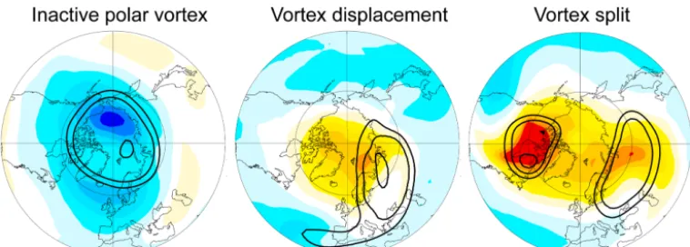
There are two main types of SSW: displacement events in which the stratospheric polar vortex is displaced from the pole andsplitevents in which the vortex splits into two or more vortices (Fig. 1). Some SSWs are a combination of both types. There are a number of methods for determin-ing the type of SSW. We do not attempt to classify event types here; however, we do provide the filtered (and unfil-tered) absolute vorticity field at 10 hPa (see Sect. 2.3), which may enable classification of split-type SSWs according to the CP07 definition, in which the edges of the vortex are identi-fied by the location of the maximum absolute vorticity gra-dient. We also provide potential vorticity (PV) interpolated onto isentropic surfaces, and geopotential heights at 10 hPa, both of which can be used to assess vortex moment diag-nostics and determine the SSW type (Mitchell et al., 2011; Seviour et al., 2013; Waugh, 1997). We note that the vor-tex moment diagnostics detect some different dates of SSWs compared to CP07 (and these events are not included in the Compendium), but the provided data would allow classifica-tion of the included events.
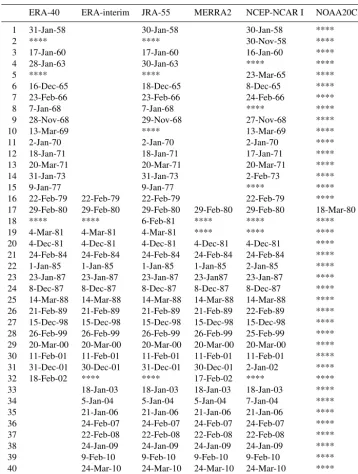
Table 2.The central dates of NH SSWs detected in each reanalysis producta. Empty cells indicate that no data are available; stars indicate that data are available but no SSW was detected.
ERA-40 ERA-interim JRA-55 MERRA2 NCEP-NCAR I NOAA20CR
1 31-Jan-58 30-Jan-58 30-Jan-58 ****
2 **** **** 30-Nov-58 ****
3 17-Jan-60 17-Jan-60 16-Jan-60 ****
4 28-Jan-63 30-Jan-63 **** ****
5 **** **** 23-Mar-65 ****
6 16-Dec-65 18-Dec-65 8-Dec-65 ****
7 23-Feb-66 23-Feb-66 24-Feb-66 ****
8 7-Jan-68 7-Jan-68 **** ****
9 28-Nov-68 29-Nov-68 27-Nov-68 ****
10 13-Mar-69 **** 13-Mar-69 ****
11 2-Jan-70 2-Jan-70 2-Jan-70 ****
12 18-Jan-71 18-Jan-71 17-Jan-71 ****
13 20-Mar-71 20-Mar-71 20-Mar-71 ****
14 31-Jan-73 31-Jan-73 2-Feb-73 ****
15 9-Jan-77 9-Jan-77 **** ****
16 22-Feb-79 22-Feb-79 22-Feb-79 22-Feb-79 ****
17 29-Feb-80 29-Feb-80 29-Feb-80 29-Feb-80 29-Feb-80 18-Mar-80
18 **** **** 6-Feb-81 **** **** ****
19 4-Mar-81 4-Mar-81 4-Mar-81 **** **** ****
20 4-Dec-81 4-Dec-81 4-Dec-81 4-Dec-81 4-Dec-81 **** 21 24-Feb-84 24-Feb-84 24-Feb-84 24-Feb-84 24-Feb-84 **** 22 1-Jan-85 1-Jan-85 1-Jan-85 1-Jan-85 2-Jan-85 **** 23 23-Jan-87 23-Jan-87 23-Jan-87 23-Jan87 23-Jan-87 **** 24 8-Dec-87 8-Dec-87 8-Dec-87 8-Dec-87 8-Dec-87 **** 25 14-Mar-88 14-Mar-88 14-Mar-88 14-Mar-88 14-Mar-88 **** 26 21-Feb-89 21-Feb-89 21-Feb-89 21-Feb-89 22-Feb-89 **** 27 15-Dec-98 15-Dec-98 15-Dec-98 15-Dec-98 15-Dec-98 **** 28 26-Feb-99 26-Feb-99 26-Feb-99 26-Feb-99 25-Feb-99 **** 29 20-Mar-00 20-Mar-00 20-Mar-00 20-Mar-00 20-Mar-00 **** 30 11-Feb-01 11-Feb-01 11-Feb-01 11-Feb-01 11-Feb-01 **** 31 31-Dec-01 30-Dec-01 31-Dec-01 30-Dec-01 2-Jan-02 ****
32 18-Feb-02 **** **** 17-Feb-02 **** ****
33 18-Jan-03 18-Jan-03 18-Jan-03 18-Jan-03 ****
34 5-Jan-04 5-Jan-04 5-Jan-04 7-Jan-04 ****
35 21-Jan-06 21-Jan-06 21-Jan-06 21-Jan-06 ****
36 24-Feb-07 24-Feb-07 24-Feb-07 24-Feb-07 ****
37 22-Feb-08 22-Feb-08 22-Feb-08 22-Feb-08 ****
38 24-Jan-09 24-Jan-09 24-Jan-09 24-Jan-09 ****
39 9-Feb-10 9-Feb-10 9-Feb-10 9-Feb-10 ****
40 24-Mar-10 24-Mar-10 24-Mar-10 24-Mar-10 ****
41 06-Jan-13 07-Jan-13 06-Jan-13 07-Jan-13 ****
aThese are the detected events in each reanalysis, but in the SSWC we provide data for all dates shown in this table for all
reanalyses.
making reanalyses highly unconstrained, the only event de-tected occurred in September 2002. This event is included in the SSWC.
2.3 Data processing
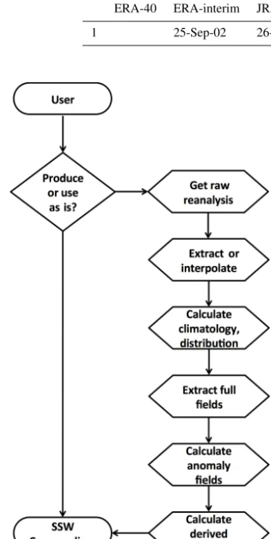
The production flowchart for the SSWC is shown in Fig. 2. We obtained the native horizontal and vertical pressure-level data for each reanalysis from various research data archives:
Figure 1.Temperature anomalies at 10 hPa (shading, (K)) and the potential vorticity at 550 K (contours shown for 75, 100, and 125 PV units) during (left) an inactive (or strong) phase of the polar vortex (∼9 January 2009), (center) a vortex displacement following the 23 January 1987 event, and (right) a vortex split following the 24 January 2009 event. MERRA2 reanalysis is used.
We extracted the following fields (when available): ver-tically integrated total column ozone; zonal winds, merid-ional winds, temperatures, geopotential heights, Ertel’s po-tential vorticity (PV), and ozone mixing ratio, on provided pressure levels; and at the surface, mean daily temperature, minimum daily temperature, maximum daily temperature, mean sea level pressure, surface pressure, total precipita-tion liquid water equivalent, and total snowfall liquid wa-ter equivalent. Most raw reanalysis output is available every 6 h (for pressure-level fields) and sometimes up to every 3 h (for surface-level fields), but we computed daily means of all fields for the SSWC. We interpolated pressure-level fields onto a 2.5◦×2.5◦latitude–longitude grid, while the surface-level fields are maintained at native horizontal resolution. We retained data on provided pressure levels, but we interpolated certain fields (PV and ozone mixing ratio) onto isentropic surfaces. Unless isentropic-level data are provided, we cal-culated potential temperature (θ) from temperature data on pressure levels using Eq. (1):
2=T p
0
p R/Cp
, (1)
where T and p are atmospheric temperature and pres-sure, respectively, p0 is a reference pressure defined as 1000 hPa, R is the molar gas constant (287 J deg−1kg−1), and cp is the specific heat capacity at constant pressure
(1004 J deg−1kg−1). The data, either on pressure or isen-tropic levels, are linearly interpolated at each time step onto 10 common isentropes (330, 350, 400, 450, 500, 550, 600, 700, 850, and 1000 K). Note that in JRA-55, isentropic-level data are provided but not at the 1000 K surface; therefore, in the SSWC missing values are indicated for this theta level.
There are two types of output provided by the SSWC: cli-matological statistics and event-based data. Clicli-matological statistic files include the mean and standard deviations of all output fields and percentiles from the climatological distri-bution for a selection of surface fields: minimum and
maxi-mum surface temperature and precipitation. The climatolog-ical statistics are defined at each spatial point for 366 days spanning 1 July–30 June. The climatological mean is based on the entire time period of each reanalysis (Table 1). To cal-culate the climatological mean, we first calcal-culate the mean of each day of the year over the full record. Then we calculate the Fourier transform of this daily mean climatology and re-tain the first four harmonics of the Fourier series (e.g., Wilks, 2006). This methodology smooths out the raw daily climatol-ogy while preserving low-frequency variability. The standard deviation is then calculated by taking the square root of the squared deviations in the raw daily data from this smoothed climatological mean. Percentiles are calculated following a method described in Zhang et al. (2005; see Eq. 1). Chosen percentiles are 5, 10, 90, and 95 %. These statistics are cal-culated using the entire data record.
Event-based files contain full field, anomaly, and derived fields for the 60 days prior to and following each SSW event in Tables 2 and 3. Anomalies are calculated using the smoothed climatology for each field, using the entire data record for each reanalysis. We caution that, while the clima-tologies for different time periods are generally quite similar, using different periods for the climatology for each reanaly-sis means that differences in reanalyreanaly-sis anomaly fields may partially be a result of the climatology chosen. In addition to full fields and anomalies, we derive a number of useful di-agnostics for understanding dynamic processes and surface climate surrounding SSW events, as described below:
1. We provide the maximum and minimum daily tempera-tures. NCEP-NCAR I provides this output; we calculate these values for the other reanalyses. Note that no in-terpolation is used – just the minimum and maximum values of the 3 or 6 hourly data – so these values may underestimate the true maximum and minimum daily temperatures.
subtract-Table 3.The central dates of the SH SSW detected in each reanalysis product.
ERA-40 ERA-interim JRA-55 MERRA2 NCEP-NCAR I NOAA20CR
1 25-Sep-02 26-Sep-02 26-Sep-02 26-Sep-02 ****
Figure 2.Flowchart showing how the SSWC can be used as is or the different steps to produce the dataset.
ing the mean and dividing by the standard deviation for the particular day of year and grid point.
3. We provide absolute vorticity (ωa) at 10 hPa. This is cal-culated from the 2.5◦×2.5◦gridded zonal and merid-ional wind fields using the vorticity equation in spheri-cal coordinates:
ωa=ζ+f = 1
a ∂v
∂λ− 1
acosφ
∂(ucosφ)
∂φ
+f, (2)
whereζis relative vorticity (defined by the parenthetical terms on the right-most side of the equation),f is the Coriolis force (2sinφ),ais the Earth’s radius,φis the latitude in radians,λis the longitude in radians,uis the zonal wind, andvis the meridional wind.
4. We provide filtered absolute vorticity at 10 hPa. Here the absolute vorticity has been subject to a spherical smoothing procedure, in which the absolute vorticity is transformed into spherical harmonic space and sub-sequently transformed back while retaining only the first 11 harmonic coefficients. This filtering is part of CP07’s event-type determination algorithm.
5. We provide zonal-mean eddy meridional heat flux (v0T0), and its wave-number 1 and 2 components, as a function of pressure level and latitude. Here the primes (0) indicate deviations from the zonal mean. These are calculated using daily data. The wave-number compo-nents are found by applying a Fourier transform to the longitude dimension.
6. We provide zonal-mean eddy meridional momentum flux (u0v0), and its wave-number 1 and 2 components, as a function of pressure level and latitude.
7. We provide the Northern Annular Mode (NAM) and the Southern Annular Mode (SAM) indices. The NAM or SAM patterns are calculated as the first empirical orthogonal function (EOF) of daily-mean zonal-mean geopotential height anomalies from 20 to 90◦N or S. The NAM or SAM indices are the principal compo-nent time series corresponding to the first EOF for each hemisphere (Baldwin and Thompson, 2009). In the stratosphere, the annular mode is related to the strength of the polar vortex; in the troposphere, the annular mode is related to shifts in the tropospheric storm tracks (Ger-ber et al., 2012; Thompson et al., 2000).
8. We provide extreme events. For each grid space, either a 0 or 1 is given if the daily precipitation, minimum tem-perature, or maximum temperature anomaly exceeds a certain threshold. For precipitation, the anomaly must exceed the 95th percentile. Temperature anomalies must either be less than the 5th or 10th percentile or greater than the 90th or 95th percentile.
10. We provide time from the SSW event at which the zonal-mean zonal wind becomes easterly, as a function of pressure and latitude.
11. We provide pressure level at which the zonal-mean zonal wind becomes easterly, as a function of time and latitude.
Finally, a number of climate indices based on independent observations (not reanalysis data) have been included to pro-vide a sense of other sources of climate variability that may be contributing to both the forcing of individual SSWs and the surface climate impacts. These include
1. measures of the phase of the El Niño–Southern Oscil-lation (ENSO). These indices allow the user to assess the state of the tropical Pacific, which has important winter effects on midlatitude climate. SSWs have been found to occur in 80 % of El Niño winters (Butler and Polvani, 2011) and may modify the El Niño telecon-nections when they occur (Butler et al., 2014; Richter et al., 2015). The Multivariate ENSO Index (MEI) is calculated as the first principal component of six different observed variables combined. The MEI data are from NOAA Physical Sciences Division (PSD): http://www.esrl.noaa.gov/psd/enso/mei/table.html. In addition to the MEI, we also provide the Oceanic Niño Index (ONI) and the Southern Oscillation Index (SOI). The ONI is calculated as the 3-month running mean of sea surface temperature anomalies in the Niño 3.4 region, based on a centered 30-year base period updated every 5 years. The ONI data are from the NOAA CPC: http://www.cpc.ncep.noaa.gov/products/ analysis_monitoring/ensostuff/detrend.nino34.ascii.txt. The SOI is calculated as the difference between the standardized sea level pressure at Tahiti and Darwin. The SOI data are from the NOAA CPC: http://www.cpc.ncep.noaa.gov/data/indices/soi. All of these indices have been linearly interpolated from monthly data to daily data, assuming the monthly values are centered on the 15th of the month;
2. the outgoing long-wave radiation Madden–Julian Oscil-lation (MJO) Index (OMI) amplitude and phase. SSWs may be related to the anomalous convection generated by the MJO during certain phases (e.g., Garfinkel et al., 2014). The OMI daily data are from NOAA PSD: http: //www.esrl.noaa.gov/psd/mjo/mjoindex/omi.1x.txt;
3. the equatorial zonal winds measured by radiosondes near the equator, provided at 10, 30, 50, and 70 hPa, as a measure of the Quasi-Biennial Oscillation (QBO). The QBO is thought to modulate the frequency of SSWs via changes in wave propagation (Baldwin et al., 2001; Dunkerton et al., 1988), perhaps in relation to the solar cycle (Labitzke et al., 2006). The QBO data are pro-vided by Freie Universitat of Berlin: http://www.geo.
fu-berlin.de/en/met/ag/strat/produkte/qbo/. These have been linearly interpolated from monthly data to daily data.
We acknowledge that other variables and indices may be use-ful for examining SSW dynamics, such as the Eliassen–Palm flux vector components or transformed Eulerian-mean diag-nostics. Some of these diagnostics could be calculated using the provided daily data on pressure levels, though this may be imprecise relative to calculations on native model levels. Model-level data are often used for analyzing transport and processes near the tropopause, where vertical resolution on provided pressure levels may be inadequate or may intro-duce interpolation errors. Regardless, the SSWC is useful for a wide range of applications, as featured in the next section.
3 Applications
Here we highlight three types of potential applications of the SSWC: (i) composite analysis, (ii) individual event analysis, and (iii) reanalysis intercomparison.
3.1 Composite analysis
Assessing the composite response to SSWs is useful for sep-arating the signals from internal noise and identifying where the signal is robust. Figure 3 shows, as a function of pres-sure level and time before and after the event, (a) zonal-mean zonal winds at 60◦N and zonal-mean temperature anomalies averaged from 50 to 90◦N, (b) the Northern Annular Mode index at each pressure level, and (c) ozone mixing ratios from 60 to 90◦N, composited over all 41 northern hemispheric SSW events (Table 2), using the JRA-55 reanalysis. Figure 4 shows the surface response composited over the 60 days fol-lowing the central date of all SSWs, including (a) mean sea level pressure anomalies, (b) surface temperature anomalies, and (c) precipitation anomalies.
Figure 3. Composites of the 60 days before and after historical SSWs in the JRA-55 reanalysis for(a)temperature anomalies aver-aged from 50–90◦N (contour levels are 2 K, bold line is 0 K) and zonal-mean zonal winds at 60◦N (shading, (m s−1)),(b)the North-ern Annular Mode (NAM) index (stdevs), and(c)ozone mass mix-ing ratio anomalies from 60 to 90◦N (ppmv).
timescales (Newman and Rosenfield, 1997). These changes near the tropopause may increase the persistence of the nega-tive NAM phase in the troposphere (Fig. 3b), potentially pro-viding a source of predictive skill for up to 60 days after the occurrence of the SSW (Maycock and Hitchcock, 2015). Fol-lowing the SSW, the stratospheric ozone over the polar cap is greatly enhanced (Fig. 3c), both due to the increased trans-port of ozone-rich air into the stratosphere via the residual mean circulation and the horizontal mixing of high-ozone air into the region as the low-ozone region of the polar vortex is moved off the pole (either in one or two lobes, depending on whether a split- or displacement-type event has occurred).
At the surface, the composite response in mean sea level pressure anomalies comprises an anomalous high over the polar cap and Greenland and an anomalous low over the
North Atlantic, a pattern that projects well onto the nega-tive phase of the NAO, the regional equivalent of the NAM (Fig. 4a). The associated surface temperature anomalies in-clude significant warming over western Greenland and east-ern Canada and strong cold air outbreaks over much of north-ern Europe, Asia, and the eastnorth-ern United States (Fig. 4b). Conditions are also anomalously wet over western and cen-tral Europe and dry over Scandinavia (Fig. 4c).
Composite analysis could also be used to consider differ-ences in SSW evolution and impacts in relation to other fac-tors, such as the differences between split- and displacement-type events, the differences between events that occur in El Niño or La Niña winters, or the different phases of the MJO. Figure 5 highlights the differences in the evolution of the 500 hPa geopotential height anomalies prior to and after a SSW during La Niña versus El Niño winters. Here we use the December–January–February ONI index to classify El Niño and La Niña years, with winters with ONI exceeding +0.5◦C defined as El Niño years and winters with ONI be-low−0.5◦C defined as La Niña years. While the sample size for these composites is small (13 events during El Niño years, 9 events during La Niña years), some major features are ap-parent; for example, the trough during El Niño and the ridge during La Niña in the North Pacific are evident throughout the evolution of the SSW. Note, however, the intensification of low-pressure anomalies in the northwest Pacific in the 60 days prior to SSWs in both El Niño and La Niña win-ters, a feature theorized in Garfinkel et al. (2012) to amplify planetary-scale waves from the troposphere into the strato-sphere and weaken the stratospheric polar vortex. During El Niño winters, the tropospheric circulation pattern is strongest over North America in the days prior to a SSW, but strongest over the North Atlantic after a SSW. During La Niña winters, the anomalies over Greenland and Europe change sign be-fore and after a SSW event, demonstrating the role of SSWs in winter climate over the North Atlantic–European region.
3.2 Individual event analysis
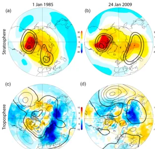
While compositing is useful for highlighting robust features of SSWs, the dynamic evolution and surface climate anoma-lies before and after each individual SSW can vary widely. The SSWC can be used to demonstrate this range of vari-ability. Figure 6 illustrates the differences in the tropospheric climate following two similar split-type SSWs, one in Jan-uary 1985 and the other in JanJan-uary 2009. In both events, the polar vortex split into two lobes: the one associated with the greatest warming anomalies centered over Canada and the other centered over northern Europe and Asia (Fig. 6a, b). The 2009 split SSW had a larger lobe that extended over most of Eurasia, but otherwise the stratospheric evolution was quite similar.
Figure 4. Composites of the 60 days after historical SSWs in the JRA-55 reanalysis for(a)mean sea level pressure anomalies (hPa), (b)surface temperature anomalies (K), and(c)precipitation anomalies (mm). The stippling indicates regions that are significantly different from the climatology at the 95 % level.
Figure 5.Composites of the 500 hPa geopotential height anomalies (m) in JRA-55 reanalysis for(a)days−60 to 0 prior to historical SSWs and(b)days 0 to+60 after historical SSWs for (top row) El Niño winters and (bottom row) La Niña winters. The stippling indicates regions that are significantly different from the climatology at the 95 % level. There are 13 events during El Niño winters and 9 events during La Niña winters. Here, if two SSWs occurred in one winter, we only considered the first event of the winter to avoid oversampling.
the 1985 event projects strongly onto the negative NAO pat-tern (Fig. 6c), with positive height anomalies over Green-land and negative height anomalies over the North Atlantic. This pattern is associated with much lower surface tempera-ture anomalies over much of Europe and Asia. However, the height anomalies in the 2 months following the 2009 split-type event do not look like the negative NAO phase, though there are weakly positive height anomalies over the Arctic
Figure 6.Comparison of two split-type SSW events,(a, c)1 January 1985 and(b, d)24 January 2009, for ERA-interim reanalysis. The top row(a, b)shows the 10 hPa temperature anomalies (shading, (K)) and the potential vorticity at 550 K (contours shown for 75, 100, and 125 PV units) at+4 days after the central date of the event. The bottom row(c, d)shows the surface temperature anomalies (shading, (K)) and the 500 hPa geopotential height anomalies (contour interval is 50 m, zero line is bold) averaged days 0–60 after the central date of the event.
official La Niña classification by the NOAA Climate Predic-tion Center by 0.1◦C), the location and strength of the North Pacific ridge during these 2 years was quite different. Other aspects of climate variability, such as the QBO, sea ice, or the MJO, may have played a role in the tropospheric climate during these time periods.
The SSWC allows easy evaluation of the spread among individual events for different features of SSWs. Figure 7 shows time series of the (a) amplitude and (b) latitude of the maximum temperature anomaly (that occurs within the range of 30–90◦ latitude and 300 to 1 hPa) and (c) the 200 hPa 40–70◦N eddy heat flux anomaly. On average, the maxi-mum temperature anomaly of ∼50 K peaks 1–2 days prior to the zonal wind reversal (Fig. 7a, bold black line), but the amplitude and timing vary substantially among the in-dividual events (colored lines), with values from 10 to al-most 100 K. Likewise, the mean latitude where the tempera-ture maximizes tends to fall between 60 and 70◦N (Fig. 7b) but ranges from ∼45◦N to the pole. The 200 hPa heat flux anomaly represents the incoming heat fluxes from the tropo-sphere via vertically propagating waves, which amplify and peak prior to the SSW (Polvani and Waugh, 2004; Sjoberg
and Birner, 2014); however, during any individual year, there may be pulses of large heat fluxes that do not result in a SSW (Fig. 7c).
3.3 Reanalysis intercomparison
Figure 7.Time series for the 30 days prior to and after the event date of major SSWs in the JRA-55 reanalysis of(a)the amplitude of the maximum temperature anomaly (within the region 30–90◦ latitude and 300 hPa to 1 hPa, (K)),(b)the latitude of the maximum temperature anomaly within that same region (degrees latitude), and (c)the anomalous eddy heat flux (K m s−1) at 200 hPa.
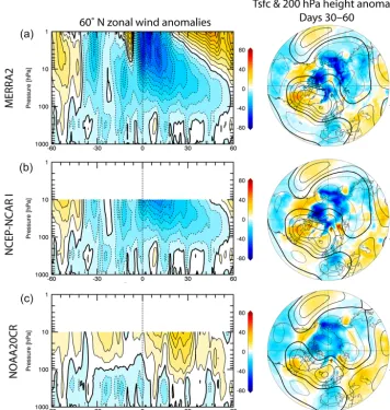
surface is constrained by assimilated observations (Fig. 8c). This means that although NOAA20CRv2c does not cap-ture the SSW event, the surface and tropospheric response contains information about the impact of this stratospheric event. Conversely, the mid- to upper-tropospheric zonal wind anomalies after the SSW event in NOAA20CRv2c are smaller (more positive) than in either NCEP1 or MERRA2, suggesting that the lack of stratospheric processes limits the
ability of this reanalysis to capture the tropospheric climate response following major breakdowns of the polar vortex.
The surface temperature anomalies and the 200 hPa geopotential height anomalies for days 30–60 after the 2013 SSW are shown in the right-hand panels of Fig. 8. In the SSWC, surface variables are provided at their native horizon-tal resolution, which is reflected in these panels in the surface temperature anomalies. MERRA2 has the highest horizontal resolution, making more regional structure and detail appar-ent. The cold anomalies over Asia and parts of the Arctic, and the tropospheric circulation anomalies at 200 hPa (par-ticularly in regions impacted by stratosphere–troposphere coupling, such as the North Atlantic), are weaker in the NOAA20CR relative to MERRA2 and NCEP1. Regional dif-ferences between all three reanalyses can be seen, particu-larly in the polar cap region where observations may not be available to constrain the reanalysis system.
4 Data usage and availability
The SSWC is designed to be a public domain product that al-lows the user either to use the data as packaged or to step into the production process and regenerate parts of the database with customized configurations. A flowchart of these options is shown in Fig. 2. For example, if the user would like to use a different set of event dates or a different climatology, they may use the provided code and documentation to extract full fields from their reanalysis product of choice and to gener-ate new anomaly and derived fields. Nonetheless, one major advantage of the SSWC is that both the full fields and the anomalies are provided (as well as the climatology), so that users can avoid downloading the terabytes of data needed to calculate the daily climatology and anomaly fields.
The SSW Compendium has been archived at NOAA’s NCEI (doi:10.7289/V5NS0RWP) in CF-compliant netCDF-4 format. The data are compressed using short integer (16-bit) packing, resulting in a full size of 300 GB for the SSWC. Some, but not all, programming platforms will properly read packed data and account for missing values. Care must be taken while reading packed data, or missing values may be unknowingly counted as finite data points.
Figure 8.Comparison of three different reanalysis products for the 7 January 2013 SSW event:(a)MERRA2,(b)NCEP-NCAR I, and (c)NOAA20CR. The left column shows 60◦N zonal-mean zonal wind anomalies (m s−1) as a function of time from the central date and pressure level. The right column shows the surface temperature anomalies (shading, (K)) and 200 hPa geopotential height anomalies (contour interval is 50 m) averaged over days 30–60 following the central date.
A subset of the SSWC can be plotted or animated at http: //www.esrl.noaa.gov/csd/groups/csd8/sswcompendium/.
The ability to readily perform (i) composite analysis, (ii) individual event analysis, and (iii) reanalysis intercom-parison is one of the main goals of the SSW Compendium. The SSWC will hopefully allow users to highlight the role of stratosphere–troposphere processes and the importance of major SSW events in winter climate and provide a compre-hensive database to compare with and improve model simu-lation of these events.
5 Summary
The SSWC database provides a simple and computationally inexpensive way to generate, download, and plot information on historical SSW events and their evolution and impacts on
daily timescales. The database is designed to be used as is, but the end user also has the ability to use the source code to customize the database to meet their specific needs. The inclusion of six different reanalysis products and a set of full, anomaly, and derived fields for every major SSW in the historical record allows several different applications of the SSWC. The ability to readily perform (i) composite analysis, (ii) individual event analysis, and (iii) reanalysis intercom-parison for projects such as S-RIP will hopefully allow users to highlight the role of stratosphere–troposphere processes and the importance of major SSW events in winter climate and provide a comprehensive database to compare with and improve model simulation of these events.
Acknowledgements. This work was funded by the NOAA Climate Program Office.
Edited by: G. König-Langlo
Reviewed by: W. Seviour and one anonymous referee
References
Baldwin, M. P. and Dunkerton, T. J.: Stratospheric Harbingers of Anomalous Weather Regimes, Science, 294, 581–584, doi:10.1126/science.1063315, 2001.
Baldwin, M. P. and Thompson, D. W. J.: A critical comparison of stratosphere-troposphere coupling indices, Q. J. Roy. Meteor. Soc., 135, 1661–1672, doi:10.1002/qj.479, 2009.
Baldwin, M. P., Gray, L. J., Dunkerton, T. J., Hamilton, K., Haynes, P. H., Randel, W. J., Holton, J. R., Alexander, M. J., Hirota, I., Horinouchi, T., Jones, D. B. A., Kinnersley, J. S., Marquardt, C., Sato, K., and Takahashi, M.: The quasi-biennial oscillation, Rev. Geophys., 39, 179–229, doi:10.1029/1999RG000073, 2001. Bosilovich, M. G., Chen, J., Robertson, F. R., and Adler, R. F.:
Eval-uation of Global Precipitation in Reanalyses, J. Appl. Meteorol. Clim., 47, 2279–2299, doi:10.1175/2008JAMC1921.1, 2008. Butler, A. H. and Polvani, L. M.: El Niño, La Niña, and
stratospheric sudden warmings: A reevaluation in light of the observational record, Geophys. Res. Lett., 38, L13807, doi:10.1029/2011GL048084, 2011.
Butler, A. H., Polvani, L. M., and Deser, C.: Separating the stratospheric and tropospheric pathways of El Niño–Southern Oscillation teleconnections, Environ. Res. Lett., 9, 024014, doi:10.1088/1748-9326/9/2/024014, 2014.
Butler, A. H., Seidel, D. J., Hardiman, S. C., Butchart, N., Birner, T., and Match, A.: Defining Sudden Stratospheric Warmings, B. Am. Meteorol. Soc., 96, 1913–1928, doi:10.1175/BAMS-D-13-00173.1, 2015.
Butler, A. H., Sjoberg, J., Seidel, D. J., and NOAA ESRL Chemical Science Division: Sudden Stratospheric Warming Compendium, Version 1.0, NOAA National Centers for Environmental Infor-mation (NCEI), doi:10.7289/V5NS0RWP, 2016.
Charlton, A. J. and Polvani, L. M.: A new look at stratospheric sud-den warmings. Part I: Climatology and modeling benchmarks, J. Climate, 20, 449–469, 2007.
Compo, G. P., Whitaker, J. S., Sardeshmukh, P. D., Matsui, N., Al-lan, R. J., Yin, X., Gleason, B. E., Vose, R. S., Rutledge, G., Bessemoulin, P., Brönnimann, S., Brunet, M., Crouthamel, R. I., Grant, A. N., Groisman, P. Y., Jones, P. D., Kruk, M. C., Kruger, A. C., Marshall, G. J., Maugeri, M., Mok, H. Y., Nordli, Ø., Ross, T. F., Trigo, R. M., Wang, X. L., Woodruff, S. D., and Worley, S. J.: The Twentieth Century Reanalysis Project, Q. J. Roy. Meteor. Soc., 137, 1–28, doi:10.1002/qj.776, 2011.
Dee, D. P., Uppala, S. M., Simmons, A. J., Berrisford, P., Poli, P., Kobayashi, S., Andrae, U., Balmaseda, M. A., Balsamo, G., Bauer, P., Bechtold, P., Beljaars, A. C. M., van de Berg, L., Bid-lot, J., Bormann, N., Delsol, C., Dragani, R., Fuentes, M., Geer, A. J., Haimberger, L., Healy, S. B., Hersbach, H., Hólm, E. V., Isaksen, L., Kållberg, P., Köhler, M., Matricardi, M., McNally, A. P., Monge-Sanz, B. M., Morcrette, J.-J., Park, B.-K., Peubey, C., de Rosnay, P., Tavolato, C., Thépaut, J.-N., and Vitart, F.: The ERA-Interim reanalysis: configuration and performance of the
data assimilation system, Q. J. Roy. Meteor. Soc., 137, 553–597, doi:10.1002/qj.828, 2011.
Dethof, A. and Hólm, E. V: Ozone assimilation in the ERA-40 reanalysis project, Q. J. Roy. Meteor. Soc., 130, 2851–2872, doi:10.1256/qj.03.196, 2004.
Dragani, R.: On the quality of the ERA-Interim ozone reanalyses: comparisons with satellite data, Q. J. Roy. Meteor. Soc., 137, 1312–1326, doi:10.1002/qj.821, 2011.
Dunkerton, T., Delisi, D., and Baldwin, M.: Distribution of Major Stratospheric Warmings in Relation to the Quasi-Biennial Oscillation, Geophys. Res. Lett., 15, 136–139, doi:10.1029/GL015i002p00136, 1988.
Fujiwara, M., Wright, J. S., Manney, G. L., Gray, L. J., Anstey, J., Birner, T., Davis, S., Gerber, E. P., Harvey, V. L., Hegglin, M. I., Homeyer, C. R., Knox, J. A., Krüger, K., Lambert, A., Long, C. S., Martineau, P., Monge-Sanz, B. M., Santee, M. L., Tegtmeier, S., Chabrillat, S., Tan, D. G. H., Jackson, D. R., Polavarapu, S., Compo, G. P., Dragani, R., Ebisuzaki, W., Harada, Y., Kobayashi, C., McCarty, W., Onogi, K., Pawson, S., Simmons, A., Wargan, K., Whitaker, J. S., and Zou, C.-Z.: Introduction to the SPARC Reanalysis Intercomparison Project (S-RIP) and overview of the reanalysis systems, Atmos. Chem. Phys. Discuss., doi:10.5194/acp-2016-652, in review, 2016. Garfinkel, C. I., Butler, a. H., Waugh, D. W., Hurwitz, M. M., and
Polvani, L. M.: Why might stratospheric sudden warmings occur with similar frequency in El Niño and La Niña winters?, J. Geo-phys. Res. Atmos., 117, D19106, doi:10.1029/2012JD017777, 2012.
Garfinkel, C. I., Benedict, J. J., and Maloney, E. D.: Impact of the MJO on the boreal winter extratropical circulation, Geophys. Res. Lett., 41, 6055–6062, doi:10.1002/2014GL061094, 2014. Gerber, E. P., Butler, A., Calvo, N., Charlton-Perez, A., Giorgetta,
M., Manzini, E., Perlwitz, J., Polvani, L. M., Sassi, F., Scaife, A. A., Shaw, T. A., Son, S.-W., and Watanabe, S.: Assessing and Understanding the Impact of Stratospheric Dynamics and Vari-ability on the Earth System, B. Am. Meteorol. Soc., 93, 845–859, doi:10.1175/BAMS-D-11-00145.1, 2012.
Gómez-Escolar, M., Calvo, N., Barriopedro, D., and Fueglistaler, S.: Tropical response to stratospheric sudden warmings and its modulation by the QBO, J. Geophys. Res.-Atmos., 119, 7382– 7395, doi:10.1002/2013JD020560, 2014.
Hoffmann, P., Singer, W., Keuer, D., Hocking, W. K., Kunze, M., and Murayama, Y.: Latitudinal and longitudinal variabil-ity of mesospheric winds and temperatures during stratospheric warming events, J. Atmos. Sol.-Terr. Phys., 69, 2355–2366, doi:10.1016/j.jastp.2007.06.010, 2007.
Kalnay, E., Kanamitsu, M., Kistler, R., Collins, W., Deaven, D., Gandin, L., Iredell, M., Saha, S., White, G., Woollen, J., Zhu, Y., Chelliah, M., Ebisuzaki, W., Higgins, W., Janowiak, J., Mo, K. C., Ropelewski, C., Wang, J., Leetmaa, A., Reynolds, R., Jenne, R., and Joseph, D.: The NCEP/NCAR 40-year reanalysis project, B. Am. Meteorol. Soc., 77, 437–471, 1996.
Spec-ifications and Basic Characteristics, J. Meteorol. Soc. Jpn., 93, 5–48, doi:10.2151/jmsj.2015-001, 2015.
Kodera, K.: Influence of stratospheric sudden warming on the equatorial troposphere, Geophys. Res. Lett., 33, L06804, doi:10.1029/2005GL024510, 2006.
Kruger, K., Naujokat, B., and Labitzke, K.: The Unusual Midwin-ter Warming in the Southern Hemisphere Stratosphere 2002, J. Atmos. Sci., 62, 603–613, 2005.
Labitzke, K. and Collaborators: The Berlin Stratospheric Data Se-ries, CD from Meteorol. Institute, Free Univ. Berlin, 2002. Labitzke, K. and Kunze, M.: Stratospheric temperatures over the
Arctic: Comparison of three data sets, Meteorol. Z., 14, 65–74, doi:10.1127/0941-2948/2005/0014-0065, 2005.
Labitzke, K., Kunze, M., and Brönnimann, S.: Sunspots, the QBO and the stratosphere in the North Polar Region – 20 years later, Meteorol. Z., 15, 355–363, doi:10.1127/0941-2948/2006/0136, 2006.
Manney, G. L., Sabutis, J. L., Pawson, S., Santee, M. L., Nau-jokat, B., Swinbank, R., Gelman, M. E., and Ebisuzaki, W.: Lower stratospheric temperature differences between meteoro-logical analyses in two cold Arctic winters and their impact on polar processing studies, J. Geophys. Res.-Atmos., 108, 8328, doi:10.1029/2001JD001149, 2003.
Manney, G. L., Schwartz, M. J., Krüger, K., Santee, M. L., Paw-son, S., Lee, J. N., Daffer, W. H., Fuller, R. A., and Livesey, N. J.: Aura Microwave Limb Sounder observations of dy-namics and transport during the record-breaking 2009 Arctic stratospheric major warming, Geophys. Res. Lett., 36, L12815, doi:10.1029/2009GL038586, 2009.
Martineau, P. and Son, S.-W.: Quality of reanalysis data during stratospheric vortex weakening and intensification events, Geo-phys. Res. Lett., 37, L22801, doi:10.1029/2010GL045237, 2010. Martineau, P., Son, S.-W., and Taguchi, M.: Dynamical consistency of reanalysis data sets in the extratropical stratosphere, J. Cli-mate, 29, 3057–3074, doi:10.1175/JCLI-D-15-0469.1, 2016. Maycock, A. C. and Hitchcock, P.: Do split and
displace-ment sudden stratospheric warmings have different annular mode signatures?, Geophys. Res. Lett., 42, 10910–943951, doi:10.1002/2015GL066754, 2015.
Mitchell, D. M., Charlton-Perez, A. J., and Gray, L. J.: Characteriz-ing the Variability and Extremes of the Stratospheric Polar Vor-tices Using 2D Moment Analysis, J. Atmos. Sci., 68, 1194–1213, doi:10.1175/2010JAS3555.1, 2011.
Molod, A., Takacs, L., Suarez, M., and Bacmeister, J.: Development of the GEOS-5 atmospheric general circulation model: evolution from MERRA to MERRA2, Geosci. Model Dev., 8, 1339–1356, doi:10.5194/gmd-8-1339-2015, 2015.
Newman, P. A. and Rosenfield, J. E.: Stratospheric ther-mal damping times, Geophys. Res. Lett., 24, 433–436, doi:10.1029/96GL03720, 1997.
Palmeiro, F. M., Barriopedro, D., García-Herrera, R., and Calvo, N.: Comparing Sudden Stratospheric Warming Definitions in Re-analysis Data, J. Climate, 28, 6823–6840, doi:10.1175/JCLI-D-15-0004.1, 2015.
Polvani, L. M. and Waugh, D. W.: Upward Wave Ac-tivity Flux as a Precursor to Extreme Stratospheric Events and Subsequent Anomalous Surface Weather Regimes, J. Climate, 17, 3548–3554, doi:10.1175/1520-0442(2004)017<3548:UWAFAA>2.0.CO;2, 2004.
Richter, J., Deser, C., and Sun, L.: Effects of stratospheric variabil-ity on El Niño teleconnections, Environ. Res. Lett., 10, 124021, doi:10.1088/1748-9326/10/12/124021, 2015.
Schoeberl, M. R.: Stratospheric warmings: Observations and theory, Rev. Geophys., 16, 521, doi:10.1029/RG016i004p00521, 1978. Schoeberl, M. R. and Hartmann, D. L.: The Dynamics of the
Strato-spheric Polar Vortex and Its Relation to Springtime Ozone De-pletions, Science, 251, 46–52, doi:10.1126/science.251.4989.46, 1991.
Seviour, W. J. M., Mitchell, D. M., and Gray, L. J.: A prac-tical method to identify displaced and split stratospheric polar vortex events, Geophys. Res. Lett., 40, 5268–5273, doi:10.1002/grl.50927, 2013.
Sjoberg, J. P. and Birner, T.: Stratospheric wave-mean flow feed-backs and sudden stratospheric warmings in a simple model forced by upward wave-activity flux, J. Atmos. Sci., 71, 4055– 4071, doi:10.1175/JAS-D-14-0113.1, 2014.
Thompson, D. W. J., Wallace, J. M., and Hegerl, G. C.: An-nular Modes in the Extratropical Circulation. Part II: Trends, J. Climate, 13, 1018–1036, doi:10.1175/1520-0442(2000)013< 1018:AMITEC>2.0.CO;2, 2000.
Uppala, S., Kallberg, P., Simmons, A., Andrae, U., Bechtold, V., Fiorino, M., Gibson, J., Haseler, J., Hernandez, A., Kelly, G., Li, X., Onogi, K., Saarinen, S., Sokka, N., Allan, R., Anders-son, E., Arpe, K., Balmaseda, M., Beljaars, A., Van De Berg, L., Bidlot, J., Bormann, N., Caires, S., Chevallier, F., Dethof, A., Dragosavac, M., Fisher, M., Fuentes, M., Hagemann, S., Holm, E., Hoskins, B., Isaksen, L., Janssen, P., Jenne, R., McNally, A., Mahfouf, J., Morcrette, J., Rayner, N., Saunders, R., Simon, P., Sterl, A., Trenberth, K., Untch, A., Vasiljevic, D., Viterbo, P., and Woollen, J.: The ERA-40 re-analysis, Q. J. Roy. Meteor. Soc., 131, 2961–3012, doi:10.1256/qj.04.176, 2005.
Van Loon, H., Jenne, R. L., and Labitzke, K.: Zonal har-monic standing waves, J. Geophys. Res., 78, 4463–4471, doi:10.1029/JC078i021p04463, 1973.
Waugh, D. N. W.: Elliptical diagnostics of stratospheric po-lar vortices, Q. J. Roy. Meteor. Soc., 123, 1725–1748, doi:10.1002/qj.49712354213, 1997.
Wilks, D. S.: Statistical Methods in the Atmospheric Sciences, 2nd Edn., Academic Press, London, 2006.