A numerical treatment of a reaction-diffusion model of spatial
pat-tern in the embryo
S. Toubaei
Islamic Azad University, Ahvaz Branch, Ahvaz, Iran. E-mail: [email protected]
M. Garshasbi∗
School of Mathematics, Iran University of Science and Technology, Tehran, Iran. E-mail: m [email protected]
M. Jalalvand
Department of Mathematics, Shahid Chamran University of Ahvaz, Ahvaz, Iran. E-mail: [email protected]
Abstract In this work the mathematical model of a spatial pattern in chemical and biological systems is investigated numerically. The proposed model considered as a nonlinear reaction-diffusion equation. A computational approach based on finite difference and RBF-collocation methods is conducted to solve the equation with respect to the appropriate initial and boundary conditions. The ability and robustness of the numerical approach is investigated using two test problems.
Keywords. Reaction-Diffusion, ecological systems, RBF collocation.
2010 Mathematics Subject Classification. 65L05, 34K06, 34K28.
1. Introduction
Generally in science phenomenon is used to discuss any sign or objective symptom; any observable occurrence or fact. Recenely geo-referenced objects and phenomena changing over time enjoy a lot of attention. Cadastral information systems with the need to record history of land parcels existence and ownership, navigational systems computing possible routes of vehicles in time, and environmental applications deal-ing with forecast prediction, especially in ”sensitive” areas with typhoon and cyclone problems, are some substantial examples of this new application area [14,17]. Identi-fying the complex relationships between ecological patterns and processes is a crucial task. One of the central issues in developmental biology is the understanding of the emergence of structure and form from the almost uniform mass of dividing cells that constitutes the early embryo. Although genes play a key role, genetics says noth-ing about the actual mechanisms which brnoth-ing together the constituent parts into a coherent pattern [11,15,14]
Qualitatively and quantitatively, mathematical models play a vital role in analyzing ecological systems. In [15] the author demonstrated, theoretically, that a system of
Received: 2 August 2016 ; Accepted: 14 November 2016.
∗Corresponding author.
reacting and diffusing chemicals could spontaneously evolve to spatially heterogeneous patterns from an initially uniform state in response to infinitesimal perturbations. In this study it is shown that diffusion could drive a chemical system to instability, leading to spatial pattern where no prior pattern existed. The author considered a system of two chemicals, in which one was an activator and the other an inhibitor. He showed that if the diffusion of the inhibitor was greater than that of the activator, then diffusion-driven instability could result [11,15].
Today the reaction-diffusion equations are widely used as models for spatial effects in ecology. They support three important types of ecological phenomena. These mod-els emphasize that simple organism movement can produce striking largescale patterns in homogeneous environments and that in heterogeneous environments, movement of multiple species can change the outcome of competition or predation [2]. Reaction-diffusion invasion models exhibit more striking behavior when population growth is not exponential but instead is regulated by density-dependent mortality. These mod-els produce travelling waves of invaders that spread out from their ”beachhead” at a constant velocity and shape.
Usually finding the exact solution of reaction-diffusion equations specially the non-linear equations is a complex task and in a lot of nonnon-linear PDE problems, one can not solve them analytically. In recent years considerable studies has been done in the numerical solution of nonlinear PDEs. The investigation of exact and numerical so-lutions for nonlinear partial differential equations (NLPDEs) plays an important role in the study of nonlinear physical phenomena. These solutions when they exist can help one to well understand the mechanism of the complicated physical phenomena and dynamical processes modelled by these nonlinear evolution equations.
In this paper the radial basis functions (RBF) collocation method and finite differ-ence approach are used to solve a system of nonlinear reaction-diffusion model arises from the chemical systems.
Meshless methods based on the collocation method have been dominant and effi-cient. Considerable studies can be found regards to the application of RBF functions for solving PDE problems in literature [3,4,6,7,8,10,9,18]. Numerical studies illus-trates the advantages of using this mesh-less methods to solve initial and/or boundary value problems [9,10]. The large number of recent research works on mesh-less meth-ods especially RBF collocation method for solving nonlinear PDE’s demonstrates the popularity that the methods have recently enjoyed.
This paper is organized as follows:
In section 2, the mathematical formulation of a spatial pattern in chemical and biological systems is presented. In section 3, a general form of the model introduced in section 2 is considered with appropriate initial and boundary conditions and a numerical procedure based on finite difference and RBF methods is established to solve this problem. Section 4 contains some test problems.
2. Reaction-diffusion modelling
no chemical F. Therefor, there will be no reaction. Now if one seeds the reaction domain with someF at various local sites and ifEcan diffuse butF be immobilized, reaction will only occur where there has been seeding, with high concentrations ofF building up at these points. Eventually,Ewould disappear and we would be left with ”spots” ofF. However, with this assumption that there is a supply of E across the domain and also a decay step forF to limit its growth, it is possible to get a balance between supply and diffusion away ofE balancing the decay ofF in the spots, to give steady-state, long-lived pattern, with highEconcentrations in between the spots and highF concentration in the spots [11]. For mathematical modelling of these systems, generally the following reaction-diffusion equation is obtained [11,14]
∂u ∂t =D
∂2u
∂x2 +F(x, t, u, c), (2.1)
where u is a vector representing chemical concentrations, D denotes the matrix of diffusion coefficients (assumed constant), and the second term represents chemical reactions, with kinetic parametersc, such as rate constants, production and degrada-tion terms. The form of theF = (f, g) have been made and studied for many specific forms [5, 11,12,16].
Here we focus on a two-chemical system, in whichu= (u1, u2) denotes the chemical
concentrations andF = (f, g) has the specific forms of the kineticsf andg[11,12,16]. As reported in [11], when a sequence of reactions are occurred as follows
XE, 2X+Y →3X, F →Y, (2.2)
according to the law of mass action, the production ofX may occur at the rate
k1a−k1u+k3u21u2. (2.3)
Furthermore the production ofY can occur at the rate
k4b−k3u21u2, (2.4)
where u1, u2, a and b are the concentrations of X, Y, E and F, respectively, and
k1, ..., k4are rate constants. Now if one assumes that X andY diffuse with diffusion
coefficientsD1 and D2 respectively, and that E and F are in abundance so that a
andbcan be assumed approximately constant, the reaction diffusion system satisfied byu1 andu2 may be written as
∂u1 ∂t =D1
∂2u1
∂x2 +k1a−k1u+k3u21u2
∂u2 ∂t =D2
∂2u 2
∂x2 +k4b−k3u21u2
. (2.5)
3. Numerical solution
Consider the equation (2.5) in more general form to be solved over in domain Ω = [0,1]×[0,1] with enclosing initial and boundary conditions
∂u1
∂t =D1 ∂2u
1
∂x2 −k1u+k3u 2
1u2+F(x, t), (x, t)∈Ω, (3.1)
∂u2
∂t =D2 ∂2u2
∂x2 −k3u 2
1u2+G(x, t), (x, t)∈Ω, (3.2)
u1(x,0) =f(x), (3.3)
u2(x,0) =g(x), (3.4)
∂u1
∂x(0, t) =ϕ1(t), (3.5)
∂u1
∂x(1, t) =ψ1(t), (3.6)
∂u2
∂x(0, t) =ϕ2(t), (3.7)
∂u2
∂x(1, t) =ψ2(t), (3.8)
It is considered that all functions in this problem areL2known functions. To establish
our proposed numerical procedure first we discretize the equations (3.1) and (3.2) by using the forward difference rule for time derivatives and the well known Crank-Nicolson scheme for other terms between successive time levelsnandn+ 1. Suppose ∆t denotes the time step size, tn = t0 +n∆t, U1n = u1(x, tn), U2n = u2(x, tn),
F(x, tn) =Fn andG(x, tn) =Gn. Discretizing these equations obtains
U1n+1−U1n
∆t = D1
U1nxx+1+U1nxx
2 −k1
U1n+1+U1n
2
+k3
(U2 1)
n+1
U2n+1+ (U12) n
U2n
2 +F
n, (3.9)
U2n+1−U2n
∆t = D2
U2nxx+1+U2nxx
2 −k3
(U12) n+1
U2n+1+ (U12) n
U2n
2
+Gn. (3.10)
By linearizing the nonlinear terms using the following formula which readily obtained by applying the Taylor expansion [13]
(U V)n+1 =Un+1Vn+UnVn+1−UnVn. (3.11)
The equations (3.9) and (3.10) may reform as
2U1n+1−D1∆tU1nxx+1+k1∆tU1n+1−k3∆t(2U1nU n 2U
n+1
1 + (U
n 1)
2Un+1
2 )
= 2U1n+D1∆tU1nxx−k1∆tU1n−k3∆t(U1n) 2Un
2 +F
n, (3.12)
2U2n+1−D2∆tU2nxx+1+k3∆t(2U1nU n 2U
n+1
1 + (U
n 1)
2Un+1
2 )
= 2U2n+D2∆tU2nxx+k3∆t(U1n) 2Un
2 +G
3.1. The RBF collocation approach. In this section, a computational procedure based on the collocation and RBF expansion methods is established to solve the problem (3.12)-(3.13) with respect to the initial an boundary conditions (3.3)-(3.8).
At collocation points xi, i = 0,1, ..., N over [0,1] such that xi, i = 1, ..., N −1
are interior points and xi, i = 0, N are boundary points, we apply the following
approximation
u1(x, tn) =U1n' N
X
j=0
λnjφ(rj), u2(x, tn) =U2n ' N
X
j=0
γjnφ(rj), (3.14)
wherenis the number of time iterations,N is the number of the data points,λn j and
γjn, j= 0,1, ..., N,are the unknown coefficients to be determined later,rj =|x−xj|
is the Euclidean norm between the pointsxandxj. The functionφ(r) can be used as
different RBFs such asφ(r) =√r2+ε2 (MQ) or φ(r) = √ 1
r2+ε2 (IMQ). In sequence
our computations are conducted based on MQ functions.
The coefficients λnj and γjn, j = 0,1, ..., N in equation (3.14) can be determined using collocation approach. To this end for each time iterationn= 1,2, ...,the 2N+ 2 unknown coefficients need to be determined from the boundary conditions given at x0 and xN and collocating U1n and U2n at the remaining N −1 distinct uniformly
distributed interior pointsxi in [x1, xN−1] as
u1(xi, tn) =U1ni' N
X
j=0
λnjφ(rij), u2(xi, tn) =U2ni' N
X
j=0
γjnφ(rij), (3.15)
whererij =|xi−xj|. Computing the first and second derivatives of the approximate
solutions and substituting the equations (3.15) into equations (3.12) and (3.13) at the collocation pointsxiand using the boundary conditions one may obtain the following
linear equations
{2 +k1∆t−2k3∆t( N
X
j=0
λnjφ(rij))( N
X
j=0
γjnφ(rij)}{ N
X
j=0
λnj+1φ(rij)}
−D1∆t N
X
j=0
λnj+1φ00(rij)−k3∆t( N
X
j=0
λnjφ(rij))2( N
X
j=0
γjn+1φ(rij))
=Fin+ (2−k1∆t) N
X
j=0
λnjφ(rij) +D1∆t N
X
j=0
λnjφ00(rij)
−k3( N
X
j=0
λnjφ(rij))2( N
X
j=0
{2 +k3∆t( N
X
j=0
λnjφ(rij))2}{ N
X
j=0
γjn+1φ(rij)} −D2∆t N
X
j=0
γjn+1φ00(rij)
+2k3∆t( N
X
j=0
λnjφ(rij))( N
X
j=0
γjnφ(rij))( N
X
j=0
λnj+1φ(rij))
=Gni + (2 +k3∆t( N
X
j=0
λnjφ(rij))2)( N
X
j=0
γjnφ(rij))
+D2∆t N
X
j=0
γjnφ00(rij), i= 1, ..., N−1. (3.17)
Furthermore according to the boundary conditions one may write
N
X
j=0
λnj+1φ0(r0j) = ϕ1(tn+1), (3.18)
N
X
j=0
λnj+1φ0(rN j) = ψ1(tn+1), (3.19)
N
X
j=0
γjn+1φ0(r0j) = ϕ2(tn+1), (3.20)
N
X
j=0
γjn+1φ0(rN j) = ψ2(tn+1). (3.21)
Equations (3.16)-(3.21) determine a system of (2N+2)(2N+2) linear equations which can be written as
AXn+1=b, (3.22)
where
Xn+1= [λn0+1, λn1+1,· · ·, λNn+1, γ0n+1, γ1n+1,· · · , γNn+1], (3.23)
and the elements of the coefficient matrixAand the right hand side vectorbcan be easily read from the equations (3.16)-(3.21). Here the singular value decomposition (SVD) approach is used to solve the equation (3.22).
4. Numerical Experiments
In this section, we implement the proposed method to solve the model equations presented in Section 2 based on MQ functions.
To investigate the ability and effectiveness of the proposed method, two numerical examples are considered. The discreteL2 andL∞ error norms by using differences
solution is known, the following error norms will be used to measure the error between the analytical and numerical solutions
L2 =
v u u th
N
X
j=0
|Uexactj −U j
appr|2, (4.1)
L∞ = max
j |U j
exact−U j
appr|, (4.2)
at the data pointsxjwhereh= N1. In the concept of RBFs it had been shown that the
accuracy of the RBFs solution, depends heavily on the choice of the shape parameter ε spatially in the MQ or inverse IMQ basis functions. Recently some authors have focused on determination of optimal values for the shape parameters in RBFs for some special problems [3,4]. Determination of suitable shape parameter is extracted experimentally for the RBFs used in this study. In our experiments the optimal value of ε is to be found numerically for each radial basis function and for each problem separately.
Example 1. In the problem (3.1)-(3.8) let
D1= 1, D2= 1, k1= 1, k3= 1,
f(x) = 2 + 1
1 +ex, ϕ1(t) =−
e3t
(1 +e3t)2, ψ1(t) =−
e1+3t
(1 +e1+3t)2,
g(x) = x
1 +ex, ϕ2(t) =
1−e3t(−1 +t)
(1 +e3t)2 , ψ2(t) =
1−e1+3tt
(1 +e1+3t)2.
With these assumptions the exact solutions are considered as
u1(x, t) = 2 +
1
1 +e3t+x, u2(x, t) =
t+x 1 +e3t+x.
The functionsF(x, t) andG(x, t) can be extracted form the exact solutions. This numerical example is studied by using mesh sizeh= 0.05 and the time step ∆t= 0.01.
Tables1and 2respectively report the L2 andL∞ error norms between the exact
and approximateu1andu2 at some time levels and for some shape parameters.
Throughout the simulation, theL∞ andL2error norms decrease with the smaller
time step size. Nevertheless increasing time levels, degrease the accuracy of the solu-tions. The behavior ofL2-error norm at t= 0.5 for computingu1 andu2 are shown
Table 1. The values of L∞ and L2 error norms versus the shape
parameter in Example 1 at some times foru1.
Time RBF shape parameterε L∞ error norm L2 error norm
0.25 2.0976×10⁻² 3.9831×10⁻²
0.3 MQ 0.45 4.0554×10⁻³ 5.6789×10⁻³
0.65 3.4831×10⁻⁴ 4.8876×10⁻⁴
0.95 1.6641×10⁻² 3.0643×10⁻²
0.25 4.6973×10⁻² 5.3856×10⁻²
0.5 MQ 0.45 8.6754×10⁻³ 9.9759×10⁻³
0.65 7.8841×10⁻⁴ 8.8996×10⁻⁴
0.95 3.9641×10⁻² 4.4843×10⁻³
0.25 7.0976×10⁻² 8.8831×10⁻² 0.7 MQ 0.45 9.0754×10⁻² 9.9779×10⁻² 0.65 3.2841×10⁻³ 4.8906×10⁻³ 0.95 8.9641×10⁻² 9.0643×10⁻²
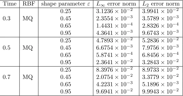
Table 2. The values of L∞ and L2 error norms versus the shape
parameter in Example 1 at some times foru2.
Time RBF shape parameterε L∞ error norm L2 error norm
0.25 3.1236×10⁻² 3.9941×10⁻²
0.3 MQ 0.45 2.3554×10⁻³ 3.5789×10⁻³
0.65 1.4431×10⁻⁴ 2.8326×10⁻⁴
0.95 4.3641×10⁻³ 9.6743×10⁻³
0.25 4.7893×10⁻² 5.2836×10⁻² 0.5 MQ 0.45 6.6754×10⁻³ 7.9756×10⁻³ 0.65 5.8741×10⁻⁴ 6.8456×10⁻⁴
0.95 2.3641×10⁻² 3.2843×10⁻²
0.25 8.3976×10⁻² 8.9733×10⁻²
0.7 MQ 0.45 2.0754×10⁻² 3.3779×10⁻²
0.65 4.2231×10⁻³ 5.1896×10⁻³ 0.95 9.6941×10⁻² 9.9943×10⁻²
Example 2. In the problem (3.1)-(3.8) let
D1= 4, Dv = 1, k1= 2, k3= 2,
F(x, t) = 4 sinh(3t+x) tanh2(3t+x) + sech2(3t+x) 3 + 8 tanh3(3t+x) ,
G(x, t) = 6 cosh(3t+x)−2(1 + 3 cosh(3t+x)) tanh3(3t+x)
+ sech2(3t+x) 3 + 2 tanh3(3t+x),
f(x) = tanh(x), ϕ1(t) = sech2(3t), ψ1(t) = sech2(1 + 3t),
g(x) = 2 sinh(x) + tanh(x), ϕ2(t) = 2 cosh(3t) + sech2(3t),
Figure 1. TheL2-error norm between the exact and approximate
solutions foru1(x, t) with respect to the shape parameterεatt= 0.5
for Example 1.
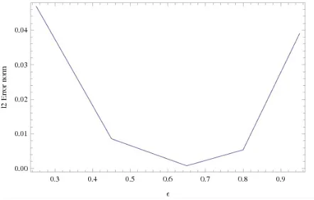
Figure 2. TheL2-error norm between the exact and approximate
solutions foru2(x, t) with respect to the shape parameterεatt= 0.5
for Example 1.
With these assumptions the exact solutions can be obtained as
u1(x, t) = tanh(3t+x), u2(x, t) = 2 sinh(3t+x) + tanh(3t+x).
This numerical example is studied by using mesh sizeh= 0.05 and the time step ∆t= 0.01.
Tables3and 4respectively demonstrate the L∞ andL2 error norms between the
exact and approximateu1andu2at some time levels and for some shape parameters.
Table 3. The values of L∞ and L2 error norms versus the shape
parameter in Example 2 at some times foru1.
Time RBF shape parameterε L∞ error norm L2 error norm
0.15 1.3462×10⁻³ 1.9833×10⁻³
0.3 MQ 0.35 7.3454×10⁻³ 9.8989×10⁻³
0.55 5.3431×10⁻² 5.0876×10⁻²
0.75 8.5641×10⁻² 9.9643×10⁻²
0.15 3.3173×10⁻³ 3.8836×10⁻³
0.5 MQ 0.35 8.8854×10⁻³ 9.9959×10⁻³
0.55 7.3441×10⁻² 8.0996×10⁻²
0.75 9.0964×10⁻² 9.9893×10⁻²
0.15 7.4576×10⁻³ 8.8981×10⁻³ 0.7 MQ 0.35 2.0754×10⁻² 3.1977×10⁻² 0.55 8.0841×10⁻² 9.1890×10⁻² 0.75 4.9741×10⁻¹ 5.1645×10⁻¹
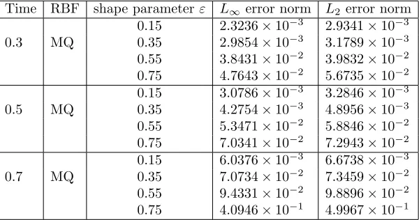
Table 4. The values of L∞ and L2 error norms versus the shape
parameter in Example 2 at some times foru2.
Time RBF shape parameterε L∞ error norm L2 error norm
0.15 2.3236×10⁻³ 2.9341×10⁻³
0.3 MQ 0.35 2.9854×10⁻³ 3.1789×10⁻³
0.55 3.8431×10⁻² 3.9832×10⁻²
0.75 4.7643×10⁻² 5.6735×10⁻² 0.15 3.0786×10⁻³ 3.2846×10⁻³
0.5 MQ 0.35 4.2754×10⁻³ 4.8956×10⁻³
0.55 5.3471×10⁻² 5.8846×10⁻²
0.75 7.0341×10⁻² 7.2943×10⁻²
0.15 6.0376×10⁻³ 6.6738×10⁻³ 0.7 MQ 0.35 7.0734×10⁻² 7.3459×10⁻² 0.55 9.4331×10⁻² 9.8896×10⁻²
0.75 4.0946×10⁻¹ 4.9967×10⁻¹
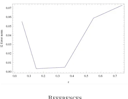
time levels, degrease the accuracy of the solutions. The behavior ofL2-error norm at
t= 0.5 for computingu1 andu2are shown in Figures3 and4.
5. Conclusion
Figure 3. TheL2-error norm between the exact and approximate
solutions foru1(x, t) with respect to the shape parameterεatt= 0.5
for Example 2.
Figure 4. TheL2-error norm between the exact and approximate
solutions foru2(x, t) with respect to the shape parameterεatt= 0.5
for Example 2.
References
[1] R. S. Cantrell and C. Cosner,Spatial Ecology via Reaction-Diffusion Equations, Wiley, Chich-ester, 2003.
[2] C. Cosner,Reaction-Diffusion Equations and Ecological Modeling Tutorials in Mathematical Biosciences IV,Lect. Not. Math.,1922(2008), 77–115.
[3] G. E. Fasshauer, J. G. Zhang,On choosing optimal shape parameters for RBF approximation, Numer. Algor., 45 (2007), 345–368. DOI 10.1017/CBO9780511791253.
[4] B. Fornberg , C. Piret,On choosing a radial basis function and a shape parameter when solving a convective PDE on a sphere, J. Comput. Phys., 227 (2008), 2758–2780.
[6] Y. C. Hon, R. Schaback,On unsymmetric collocation by radial basis functions, Appl. Math. Comput., 119 (2001), 177–186.
[7] S. Hubbert, Closed form representations for a class of compactly supported radial basis functions, Adv. Comput. Math., 36 (2012), 115–136.
[8] E. J. Kansa, Multiquadrics,A scattered data approximation scheme with applications to com-putational fluid-dynamics, I Surface approximations and partial derivative estimates, Comput. Math. Appl., 19 (1990), 127–145.
[9] A. La Rocca, A. Hernandez Rosales and H. Power,Radial basis function Hermite collocation approach for the solution of time dependent convectiondiffusion problems, Engin. Anal. Bound. Elem., 29 (2005), 359–370.
[10] J. Li, A. H. D. Cheng, C. S. Chen,A comparisons of efficiency and error convergence of mul-tiquadric collocation method and finite element method, Eng. Anal. Bound. Elem., 27 (2003), 251–257.
[11] P. K. Maini, K. J. Paintera, H. N. P. Chaub,Spatial pattern formation in chemical and biological systems, J. Chem. Soc., Faraday T rans., 93 (1997), 3601–3610.
[12] G. Nicolis, I. Prigogine,Self-Organization in Non-Equilibrium Systems: From Dissipative Struc-tures to Order Through Fluctuations, Wiley, New York, 1977.
[13] S. G. Rubin, R.A. Graves,Cubic Spline Approximation for Problems in Fluid MechanicsNasa TR R-436, Washington, D.C., 1975.
[14] N. Tryfona,Modeling Phenomena in Spatiotemporal Databases: Desiderata and Solutions, Lec-ture Notes in Computer Science, Springer-Verlag, 2006.
[15] A. M. Turing,Philosophical Transactions of the Royal Society of London.Series B, Biol. Sci., 237 (1952), 37–72.
[16] M. J. Ward, Asymptotic Methods for Reaction-Diffusion Systems: Past and Present, Bull. Math. Bio., 68 (2006), 1151–1167.
[17] M. Worboys,A Unified Model for Spatial and Temporal Information., The Computer Journal, 37 (1994), 26–34.