Vol. 5, No. 2, (2015), pp 11-28
The block LSMR algorithm for solving
linear systems with multiple
right-hand sides
F. Toutounian∗ and M. Mojarrab
Abstract
LSMR (Least Squares Minimal Residual) is an iterative method for the solution of the linear system of equations and least-squares problems. This paper presents a block version of the LSMR algorithm for solving linear sys-tems with multiple right-hand sides. The new algorithm is based on the block bidiagonalization and derived by minimizing the Frobenius norm of the resid-ual matrix of normal equations. In addition, the convergence of the proposed algorithm is discussed. In practice, it is also observed that the Frobenius norm of the residual matrix decreases monotonically. Finally, numerical ex-periments from real applications are employed to verify the effectiveness of the presented method.
Keywords: LSMR method; Bidiagonalization; Block methods; Iterative methods; Multiple right-hand sides.
1 Introduction
This paper is concerned with the solution of linear system of the form
AX=B, A∈Rn×n, B∈Rn×s, s≪n. (1)
If A is large and sparse or sometimes not readily available, then iterative solvers may become the only choice. These solvers are categorized to the following three classes:
∗Corresponding author
Received 23 April 2014; revised 6 August 2014; accepted 18 March 2015 F. Toutounian
Department of Applied Mathematics, Faculty of Mathematical Sciences, Ferdowsi Univer-sity of Mashhad, Iran.
The Center of Excellence on Modelling and Control Systems, Ferdowsi University of Mash-had, Iran. e-mail: [email protected]
M. Mojarrab
Department of Applied Mathematics, Faculty of Mathematical Sciences, Ferdowsi Univer-sity of Mashhad, Iran.
Department of Mathematics, University of Sistan and Baluchestan, Zahedan, Iran. email: [email protected]
The first class is the global methods. The term global is due to Saad [34] and has been further expanded by Jbilou et al. [21] with the global FOM and GMRES algorithms for matrix equations. These methods are based on the use of a global projection process onto a matrix Krylov subspace. References on this class include [2, 7, 8, 12, 13, 13, 21–23, 25–27, 32, 33].
The second class is the seed methods. The main idea of this kind of methods is briefed below. We first select a single system as the seed system and generate the corresponding Krylov subspace. Then we project all the residuals of the other linear systems onto the same Krylov subspace to find new approximate solutions as initial approximations. See [3,5,7,18,20,30,35] for details.
The last class is the block methods which are more suitable for dense systems with preconditioner. The first block solvers are the block conjugate gradient (Bl-CG) algorithm and the block biconjugate gradient (Bl-BCG) al-gorithm proposed in [28]. Variable Bl-CG alal-gorithms for symmetric positive definite problems are implemented on parallel computers [19, 29]. If the ma-trix is symmetric, an adaptive block Lanczos algorithm and a block version of Minres method are devised in [17]. For nonsymmetric problems, the Bl-BCG algorithm [6, 28], the block generalized minimal residual (Bl-GMRES) algo-rithm [1, 1, 4, 7, 9–11, 36, 37], the block quasi minimum residual (Bl-QMR) al-gorithm [14], the block BiCGStab (Bl-BICGSTAB) alal-gorithm [31], the block Lanczos method [34] and the block least squares (Bl-LSQR) algorithm [15] have been developed.
In this paper, we present a block version of LSMR algorithm [4] for solving the problem (1). Our algorithm is based on the block bidiagonalization [9]. We construct a simple recurrence formula for generating the sequences of ap-proximations{Xk} such that the Frobenius norm ofATRk decreases mono-tonically, whereRk=B−AXk.
Throughout this paper, we use the following notations. For twon×s
matricesXandY, we define the following inner product: ⟨X, Y⟩= tr(XTY), where tr(Z) denoted the trace of the square matrixZ. The associated norm is the Frobenius norm denoted by∥ · ∥F. We will use the notation⟨·,·⟩2 for the usual inner product in Rn and the associated norm denoted by ∥ · ∥2. Finally, 0s andIs will denote the zero and the identity matrices inRs×s.
2 The LSMR algorithm
In this section, we present a brief of the LSMR algorithm [4], which is an iterative method for solving real linear system of the form
Ax=b,
whereA is a matrix of ordernandx, b∈Rn.
LSMR algorithm uses an algorithm of Golub and Kahan [10], which is stated as procedure Bidiag 1 in [32] to reduce the augmented matrix [b A] to the upper-diagonal form [β1e1 Bk], wheree1denotes the first column of the
identity matrix. The procedure Bidiag 1 can be described as follows.
Bidiag 1(Starting vectorb; reduction to lower bidiagonal form)
β1u1=b, α1v1=ATu1,
βi+1ui+1=Avi−αiui,
αi+1vi+1=ATui+1−βi+1vi, }
i= 1,2, . . . (2)
The scalarsαi ≥0 and βi ≥0 are chosen so that∥ui∥2=∥vi∥2 = 1. With
the definitions
Uk≡[u1, u2, . . . uk], Vk ≡[v1, v2, . . . , vk], Bk ≡
α1
β2 α2
. .. . ..
βk αk
βk+1
,
Lk+1= [Bk αk+1ek+1], Vk+1=
[
Vk vk+1
]
,
the recurrence relations (2) may be rewritten as
Uk+1(β1e1) =b,
AVk =Uk+1Bk,
ATUk+1=VkBkT +αk+1vk+1eTk+1=Vk+1LTk+1.
ATAVk=ATUk+1Bk=Vk+1LTk+1Bk =Vk+1
[
BkT αk+1eTk+1
]
Bk,
=Vk+1
[
BkTBk
αk+1βk+1eTk ]
.
Hence using procedure Bidiag 1 the LSMR method constructs an approxi-mation solution of the formxk =Vkykwhich solves the least-squares problem minyk∥A
Tr
k∥,whererk=b−Axk. The main steps of the LSMR algorithm can be summarized as follows.
Algorithm 1LSMR algorithm
Setβ1u1=b, α1v1 =ATu1, α1=α1,ζ1 =α1β1, ρ0= 1, ρ0= 1, c0 = 1,
s0= 0,h1=v1, h0= 0,x0= 0,
Fork= 1,2, . . ., until convergence Do:
βk+1uk+1=Avk−αkuk,
αk+1vk+1=ATuk+1−βk+1vk,
ρk= (α2k+β
2 k+1)
1 2,
ck =αk/ρk,
sk=βk+1/ρk,
θk+1=skαk+1,
αk+1=ckαk+1,
θk =sk−1ρk,
ρk= ((ck−1ρk) 2
+θ2k+1)
1 2
,
ck =ck−1ρk/ρk,
sk=θk+1/ρk,
ζk=ckζk,
ζk+1=−skζk,
hk=hk−(θkρk/
(
ρk−1ρk−1
) )hk−1,
xk=xk−1+ (ζk/(ρkρk))hk,
hk+1=vk+1−(θk+1/ρk)hk, If|ζk+1|is small enough then stop, End Do.
More details about the LSMR algorithm can be found in [4].
3 The block LSMR method
We first recall the block Bidiag 1 algorithm [9]. This algorithm is the basis for our block LSMR method.
The block Bidiag 1 procedure constructs the sets of then×sblock vectors
V1, V2, . . . andU1, U2, . . . such that ViTVj = 0s, UiTUj = 0s, fori ̸=j, and
U1B1=B, V1A1=ATU1,
Ui+1Bi+1=AVi−UiATi,
Vi+1Ai+1=ATUi+1−ViBiT+1,
}
i= 1,2, . . . , k, (3)
where Ui, Vi ∈ Rn×s;Bi, Ai ∈ Rs×s, and U1B1, V1A1, Ui+1Bi+1, Vi+1Ai+1
are thin QR decompositions of the matricesB, ATU
1, AVi−UiATi ,ATUi+1−
ViBiT+1,respectively. With the definitions
Uk≡[U1, U2, . . . , Uk], Vk ≡[V1, V2, . . . , Vk], Tk≡
AT
1
B2 AT2
. .. . ..
Bk ATk
Bk+1
,
the recurrence relations (3) may be rewritten as:
Uk+1E1B1=B,
AVk =Uk+1Tk,
ATUk+1=VkTkT +Vk+1Ak+1EkT+1,
where Ei is the (k+ 1)s×s matrix which is zero except for the rows i to
i+s, which are thes×s identity matrix. We have also VTkVk =Iks and
UTk+1Uk+1=I(k+1)s,whereIlis thel×l identity matrix. We define
Lk+1≡
[
Tk Ek+1ATk+1
]
,
then
ATUk+1=Vk+1L
T k+1,
ATAVk=ATUk+1Tk=Vk+1L
T
k+1Tk=Vk+1
[
TT
k
Ak+1EkT+1
]
Tk
=Vk+1
[
TT
kTk
Ak+1EkT+1Tk ]
. (4)
At iterationkwe seek an approximate solutionXk of the form
Xk=VkYk, (5)
whereYk is anks×smatrix. LetBk≡AkBk for allk. Since
ATRk=ATB−ATAXk
we have
ATRk =V1B1−Vk+1
[
TT
kTk
Ak+1EkT+1Tk ]
Yk
=Vk+1(E1B1−
[
TT
k Tk
Bk+1E
T k
]
Yk), (6)
whereEk is theks×smatrix, which is zero except forkthsrows, which are thes×sidentity matrix.
In the block LSMR algorithm, we would like to chooseYk∈Rks×swhich minimizes the Frobenius norm of ATRk. From (6),ATRk can be written as
ATRk =Vk+1
[ e
E1B1−TkTTkYk −Bk+1E
T kYk
]
, (7)
whereEe1 is the matrix obtained fromE1 by deleting its last block row. But
since the columns of the matrixVk+1 are orthonormal, it follows that:
∥ATRk∥2F = [
e
E1B1−TkTTkYk −Bk+1E
T kYk
]
2
F
=∥Ee1B1−TkTTkYk∥2F+∥Bk+1E T kYk∥2F.
(8) We now define the linear operatorsχk andψk as follows.
ForY ∈Rks×s
χk(Y) =TkTTkY, and
ψk(Y) =Bk+1E
T kY.
Then the relation (8) can be expressed as
∥ATRk∥2F =∥χk(Yk)−Ee1B1∥2F+∥ψk(Yk)∥2F. (9)
Therefore, Yk minimizes the Frobenius norm of the quantity ATRk if and only if it satisfies the following linear matrix equation
χTk(χk(Yk)−Ee1B1) +ψTk(ψk(Yk)) = 0s, (10)
where the linear operatorsχT
k andψ
T
k are the transpose of the operatorsχk andψk, respectively. Therefore, (10) is also written as the following
(TkTTk)T(TkTTkYk−Ee1B1) + (Bk+1E T k)
T(B k+1E
T
kYk) = 0s. (11)
Hence,Yk is given by
b
Tk = (TkTTk)2+EkB
T
k+1Bk+1E T
k, Fk =TkTTkEe1B1. (12)
We define the matrixTk as follows:
Tk=
[
TkTTk
Bk+1E
T k ] =
A1 B
T 2
B2 A2 . ..
. .. . .. BT k
Bk Ak
Bk+1
,
whereAi=AiATi +BiT+1Bi+1, fori= 1,2, . . . , k. Therefore
b
Tk =T
T
kTk, Fk= [(A1B1)T(B2B1)T0s. . .0s]T, (13)
and the approximate solution of the system (1) is given by
Xk=VkTbk−1Fk.
Suppose that using the QR decomposition [11], we obtain a unitary matrix
Qk such that
Tk=Qk
[
Rk
0s×ks ]
, Rk=
α1β2 θ3
α2 β3 θ4
. .. . .. . ..
αk−2 βk−1 θk
αk−1βk
αk , (14)
whereRk is upper triangular as shown andαi,βi,θi are thes×smatrices. So,
Xk=Vk(R
T
kRk)−1Fk. By setting
Pk=VkR−
1
k ≡
[
P1P2. . . Pk ]
,
and
Fk =R−
T k Fk ≡
[
φT1 φT2 . . . φTk ]T
,
we have
Pk = (Vk−Pk−2θk−Pk−1βk)α−
1 k ,
Xk =Xk−1+Pkφk. (15)
Rk =Rk−1−APkφk, (16) whereAPkcan be computed from the previousAPk’s andAVk by the simple update
APk= (AVk−APk−2θk−APk−1βk)α−
1 k .
In addition, as [4], we show that the ∥Rk∥F can be estimated by a simple formula. By transforming Tk to block upper-bidiagonal form using a QR
factorization: [ bRk 0
]
=Qbk+1Tk withQbk+1=Pbk. . .Pb1, we have
Rk=B−AXk
=U1B1−AVkYk
=Uk+1(E1B1−TkYk)
= ˇUk+1QbTk+1(Qbk+1E1B1−
[ bRk 0
]
Yk).
Since the columns of the matricesQbk+1 andUk+1 are orthonormal, we have
∥Rk∥F =∥Qbk+1E1B1−
[ bRk 0
]
Yk∥F. (17)
With definitions
b
Qk+1E1B1= [βe1T . . . βe T k−1 β˙
T k β¨
T k+1]
T, Rb
kY = [τe1T . . . τe T k−1τ˙
T k]
T, (18)
the following Lemma shows that we can estimate∥Rk∥F from just the last two blocks ofQbk+1E1B1 and the last block ofRbkYk.
Lemma 1. In (17)and (18),βei=τei fori= 1,2, . . . , k−1.
Proof. The proof is similar to that of Lemma 3.1 in [4] (see [28]).
For the Frobenius norm ofATRk, by using Theorem 1 (in section 4), we can also obtain the following simple formula:
∥ATRk∥2F =∥A TR
k−1∥2F− ∥φk∥2F, with ∥A TR0∥
F =∥B1∥F =∥φ0∥F.
Algorithm 2Algorithm (Bl-LSMR ) SetX0= 0n×s,
Seta0= 0s,b−1= 0s,b0=Is,c0= 0s,d−1= 0s,d0=Is, SetP−1=P0= 0n×s,
ComputeU1B1=B,V1A1=ATU1 (QR decomposition ofB andATU1),
SetB1=A1B1,
Setφ−1= 0s, φ0=−B1,
Set∥ATR0∥
F =∥φ0∥F,
Fork= 1,2, . . ., until convergence Do:
Wk =AVk−UkATk,
Uk+1Bk+1=Wk (QR decomposition ofWk),
Ak =AkATk +B
T
k+1Bk+1,
Sk =ATUk+1−VkBkT+1,
Vk+1Ak+1=Sk (QR decomposition ofSk),
Bk+1=Ak+1Bk+1,
˙
βk =dk−2B
T k, ˙
αk=ck−1β˙k+dk−1Ak,
βk =ak−1β˙k+bk−1Ak,
θk =bk−2B
T k,
Compute an unitary matrix[ Q(ak, bk, ck, dk) such that
ak bk
ck dk ] [
˙
αk
Bk+1
] =
[
αk
0 ]
,
φk=−α−kT(θ T
kφk−2+β T kφk−1),
Pk= (Vk−Pk−2θk−Pk−1βk)α−
1 k ,
Xk =Xk−1+Pkφk,
Rk =Rk−1−APkφk,
∥ATR
k∥2F =∥ATRk−1∥2F− ∥φk∥2F, If∥ATR
k∥F is small enough then stop, End Do.
The Bl-LSMR algorithm will be break down at stepk, if αk is singular.
This happens when the matrix [
˙
αk
Bk+1
]
is not full rank. So the Bl-LSMR
algorithm will not break down at stepk, ifBk+1is nonsingular. We will not
treat the problem of breakdown in this paper and we also assume that the matricesBk’s produced by the Bl-LSMR algorithm are nonsingular.
We mention that, we can use the Bl-LSMR algorithm for computing a matrix solution X to the problem
minimize∥AX−B∥F, A∈Rm×n, B∈Rm×s, s≪min{m,n},
4 The convergence of the Bl-LSMR algorithm
In this section, we aim at studying the convergence behavior of the Bl-LSMR method. We first give the following lemmas.
Lemma 2. Let Pi, i= 1,2, . . . , k, be the n×s auxiliary matrices produced
by the Bl-LSMR algorithm and Rk be the residual matrix associated with the
approximate solutionXk of the matrix equation(1). Then, we have
(ATAPk)TATRk = 0s.
Proof. UsingPk=VkR−
1
k and equation(4), we have
ATAPk=ATAPkEk
=ATAVkR −1 k Ek
=Vk+1
[
TkTTk
Bk+1E
T k
]
R−k1Ek. (19)
From (19), and (7), we have
(ATAPk)T(ATRk) =E T kR
−T k
[
TkTTk,(Bk+1E T k)
T]VT k+1Vk+1
[ e
E1B1−TkTTkYk −Bk+1E
T kYk
]
=ETkR−kT(TkTTk(Ee1B1−TkTTkYk)−(Bk+1E T k)
TB k+1E
T kYk) = 0s. (from (11))
We note thatVk+1 is orthonormal, thusV T
k+1Vk+1=I(k+1)s.
Lemma 3. Let Pi, i= 1,2, . . . , k, be the n×s auxiliary matrices produced
by the Bl-LSMR algorithm. Then we have the following property
PiTATAATAPi=Is.
(ATAPi)T(ATAPi) = (Vi+1
[
TT
i Ti
Bi+1E
T i
]
R−i1Ei)T(Vi+1
[
TT
i Ti
Bi+1E
T i
]
R−i1Ei)
=ETi R−iT
[
TT
i TiB T i+1Ei
] [ TT i Ti
Bi+1E
T i
]
R−i 1Ei
=ETi R−iTTTiTiR− T i Ei
=ETi R−iT
[
RTi 0ks×s ]
QTiQi
[
Ri
0s×ks ]
R−i 1Ei
=ETi [Iks 0ks×s ] [ Iks
0s×ks ]
Ei
=ETi Ei=Is.
Theorem 1. Let Xk be the approximate solution of (1), obtained from the
Bl-LSMR algorithm. Then
∥ATRk∥F ≤ ∥ATRk−1∥F,
whereRk=B−AXk.
Proof. From(16), we have
ATRk−1=ATRk+ATAPkφk.
Using Lemma 2, sinceATR
k andATAPk are orthogonal, we have
∥ATRk−1∥2F =∥A TR
k∥2F+∥A TAP
kφk∥2F.
Thus
∥ATRk∥2F =∥A TR
k−1∥2F− ∥A TAP
kφk∥2F.
Using Lemma 3, we have
∥ATRk∥2F =∥A TR
k−1∥2F− ∥φk∥2F, ∥ATRk∥F ≤ ∥ATRk−1∥F.
5 Numerical examples
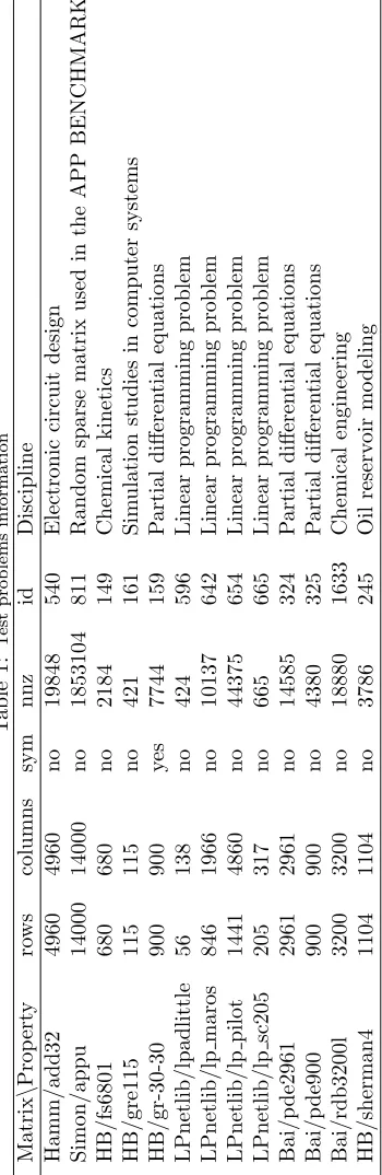
In this section, we consider the system AX =B, where A ∈ Rm×n, B ∈ Rm×s, X ∈Rn×s, and we present numerical results for several matrices taken from the University of Florida Sparse Matrix Collection (Davis [7]). These matrices with their properties are shown in Table 1. Our implementation is done on MATLAB version 07 on a PC machine with 4 GB RAM. Moreover, for the initial guessX0= 0n×sandB = rand(m, s), where the function rand creates an m×srandom matrix with the coefficients uniformly distributed in [0,1]. The stopping criteria is set to∥ATR
k∥F/∥Rk∥F ≤10−10× ∥A∥F. Diagonal scaling was applied to the columns of [A, B] to give a scaled problem AX =B, in which the columns of [A, B] have unit 2-norm. By scaling, the number of iterations of Bl-LSMR for convergence reduced satis-factorily.
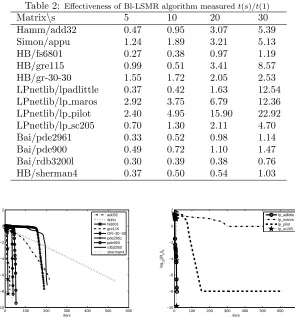
In Table 2, we give the ratiot(s)/t(1), fors= 5,10,20, and 30, wheret(s) is the CPU time for Bl-LSMR algorithm and t(1) is the CPU time obtained when applying LSMR for one right-hand side linear system. Note that the time obtained by LSMR for one right-hand side depends on which right-hand was used. So, t(1) is the average of the times needed for the s right-hand sides using LSMR. The results of Table 2 show that the Bl-LSMR algorithm is effective and less expensive than the LSMR algorithm, because the indicator
t(s)/t(1) is less than s.
To show that the Frobenius norm of residual matrix decreases monoton-ically, we display the convergence history in Figure 1 for the systems corre-sponding to the matrices of Table 2 and Bl-LSMR algorithm. In this figure, the vertical axis and horizontal axis are the logarithm in base 10 of the Frobe-nius norm of residual matrix and the number of iterations to convergence, respectively. We observe that for all matrices the Frobenius norm of residual matrix decreases monotonically.
We display the convergence history of Bl-LSMR and Bl-LSQR in Figure 2 for the system corresponding to the matrix LPnetlib/lp pilot. Figure 3 (left and right) shows both solvers reducing ∥ATR
Table 2: Effectiveness of Bl-LSMR algorithm measuredt(s)/t(1)
Matrix\s 5 10 20 30
Hamm/add32 0.47 0.95 3.07 5.39
Simon/appu 1.24 1.89 3.21 5.13
HB/fs6801 0.27 0.38 0.97 1.19
HB/gre115 0.99 0.51 3.41 8.57
HB/gr-30-30 1.55 1.72 2.05 2.53
LPnetlib/lpadlittle 0.37 0.42 1.63 12.54
LPnetlib/lp maros 2.92 3.75 6.79 12.36
LPnetlib/lp pilot 2.40 4.95 15.90 22.92
LPnetlib/lp sc205 0.70 1.30 2.11 4.70
Bai/pde2961 0.33 0.52 0.98 1.14
Bai/pde900 0.49 0.72 1.10 1.47
Bai/rdb3200l 0.30 0.39 0.38 0.76
HB/sherman4 0.37 0.50 0.54 1.03
0 100 200 300 400 500 600
−10 −8 −6 −4 −2 0 2 iters log 10 ||R k ||F add32 appu fs6801 gre115 GR−30−30 pde2961 pde900 rdb3200l sherman4
0 100 200 300 400 500 600 700
−10 −8 −6 −4 −2 0 2 iters log 10 ||R k ||F lp_adlittle lp_maros lp_pilot lp_sc205
Figure 1: Convergence history of the Bl-LSMR algorithm with s=20
0 20 40 60 80 100 120 140
−10 −8 −6 −4 −2 0 2 iters log 10 (||A TR K ||/||R k ||) Bl−LSQR Bl−LSMR
0 20 40 60 80 100 120 140
−7 −6 −5 −4 −3 −2 −1 0 1 2 iters log 10 ||R k || Bl−LSQR Bl−LSMR
6 Conclusion
In this paper, we have presented a block version of LSMR algorithm for solving linear systems with multiple right-hand sides. We derived a sim-ple recurrence formula for generating the sequence of approximate solutions
{Xk} such that the Frobenius norm of the quantity ATRk decreases mono-tonically. In addition, we studied the convergence of the presented method. Besides, we showed that in absence of the break down condition, the pre-sented algorithm always converges. Numerical results have shown that the new algorithm obtains the results which are effective and less expensive than the LSMR algorithm applied to each right-hand side.
Acknowledgements
We would like to thank the referees for their valuable remarks and helpful suggestions.
References
1. Abdel-Rehim, A. M., Morgan, R. B. and Wilcox, W.Improved seed meth-ods for symmetric positive definite linear equations with multiple
right-hand sides, 2008, Arxiv preprint arXiv:0810.0330v1.
2. Bellalij, M., Jbilou, K. and Sadok, H.New convergence results on the
global GMRES method for diagonalizable matrices, J. Comput. Appl.
Math. 219 (2008) 350-358.
3. Chan,T. F. and Wang, W.Analysis of projection methods for solving
lin-ear systems with multiple right-hand sides, SIAM J. Sci. Comput. 18
(1997) 1698-1721.
4. Chin-Lung Fong, D. and Saunders, M.LSMR: An iterative algorithm for
sparse least-squares problems, SIAM J. Sci. Comput. 33 (2011) 2950-2971.
5. Dai, H.Two algorithms for symmetric linear systems with multiple
right-hand sides, Numer. Math. J. Chin. Univ. (Engl. Ser.) 9 (2000) 91-110.
6. Darnell, D., Morgan, R. B. and Wilcox, W.Deflated GMRES for systems
with multiple shifts and multiple right-hand sides, Linear Algebra Appl.
429 (2008) 2415-2434.
7. Davis, T. A. University of Florida Sparse Matrix Collection, http://www.cise.ufl.edu/research/sparse / matrices.
8. Freund, R. and Malhotra, M.A Block-QMR algorithm for non-hermitian
linear systems with multiple right-hand sides, Linear Algebra Appl. 254
9. Golub, G. H., Luk, F. T. and Overton, M. L. A Block Lanczos method for computing the singular values and corresponding singular vectors of
the matrix, ACM Trans. Math. Software 7 (1981) 149-169.
10. Golub, G. H. and Kahan, W. Calculating the singular values and
pseu-doinverse of a matrix, SIAM J. Numer. Anal, 2 (1965) 205-224.
11. Golub, G. H. and Van Loan, C. F.Matrix Computations, Johns Hopkins University Press, Baltimore, MD, 1983.
12. Gu, G. and Cao, Z.A block GMRES method augmented with eigenvectors, Appl. Math. Comput. 121 (2001) 271-289.
13. Gu, G. and Qian, H.Skew-symmetric methods for solving nonsymmetric
linear systems with multiple right-hand sides, J. Comput. Appl. Math.
223 (2009) 567-577.
14. Gu, C. and Yang, Z.Global SCD algorithm for real positive definite linear
systems with multiple right-hand sides, Appl. Math. Comput. 189 (2007)
59-67.
15. Guennouni, A. El., Jbilou, K. and Sadok, H. A block version of
BICGSTAB for linear systems with multiple right-hand sides, Elec.
Trans. Numer. Anal. 16 (2003) 129-142.
16. Guennouni, A. El., Jbilou, K. and Sadok, H.The block Lanczos method
for linear systems with multiple right-hand sides, Appl. Numer. Math. 51
(2004) 243-256.
17. Gutknecht, M. H. Block Krylov space methods for linear systems with multiple right-hand sides: an introduction, in: A. H. Siddiqi, I. S. Duff, O. Christensen (Eds.), Modern Mathematical Models, Methods and
Al-gorithms for Real Word Systems, Anamaya Publishers, New Delhi, India,
2007, 420-447.
18. Haase, G. and Reitzinger, S.Cache issues of algebraic multigrid methods
for linear systems with multiple right-hand sides, SIAM J. Sci. Comput.
27 (2005) 1-18.
19. Heyouni, M.The global Hessenberg and global CMRH methods for linear
systems with multiple right-hand sides, Numer. Algorithms 26 (2001)
317-332.
20. Heyouni, M. and Essai, A. Matrix Krylov subspace methods for linear
systems with multiple right-hand sides, Numer. Algorithms 40 (2005)
137-156.
21. Jbilou, K., Messaoudi, A. and Sadok, H.Global FOM and GMRES
22. Jbilou, K. and Sadok, H.Global Lanczos-based methods with applications, Technical Report LMA 42, Universiti du Littoral, Calais, France, 1997.
23. Jbilou, K, Sadok, H. and Tinzefte, A. Oblique projection methods for
linear systems with multiple right-hand sides, Elec. Trans. Numer. Anal.
20 (2005)119-138.
24. Joly, P.Resolution de Systems Lineaires Avec Plusieurs Second Members
par la Methode du Gradient Conjugue, Tech. Rep. R-91012, Publications
du Laboratire d’Analyse Numerique, Universite Pierre et Marie Curie, Paris, 1991.
25. Karimi, S. and Toutounian, F.The block least squares method for solving
nonsymmetric linear systems with multiple right-hand sides, Appl. Math.
Comput. 177 (2006) 852-862.
26. Lin, Y. Implicitly restarted global FOM and GMRES for
nonsymmet-ric matrix equations and Sylvester equations, Appl. Math. Comput. 167
(2005) 1004-1025.
27. Liu, H. and Zhong, B.Simpler block GMRES for nonsymmetric systems
with multiple right-hand sides, Elec. Trans. Numer. Anal. 30 (2008) 1-9.
28. Mojarrab, M.The Block least square methods for matrix equations, PhD thesis, Ferdowsi University of Mashhad, Iran, 2014.
29. Morgan, R. B. Restarted block-GMRES with deflation of eignvalues, Appl. Numer. Math. 54 (2005) 222-236.
30. Nikishin, A. and Yeremin, A. Variable block CG algorithms for solving large sparse symmetric positive definite linear systems on parallel
com-puters I: general iterative scheme, SIAM J. Matrix Anal. 16 (1995)
1135-1153.
31. ´OLeary, D.The block conjugate gradient algorithm and related methods, Linear Algebra Appl. 29 (1980) 293-322.
32. Paige, C. C. and Saunders, M. A. LSQR: an algorithm for sparse linear
equations and sparse least squares, ACM Trans. Math. Software 8 (1982)
43-71.
33. Robbe, M. and Sadkane, M. Exact and inexact breakdowns in the block
GMRES method, Linear Algebra Appl. 419 (2006) 265-285.
34. Saad, Y. Iterative methods for sparse linear systems, SIAM, 2nd edn, 2003.
35. Saad, Y. On the Lanczos method for solving symmetric linear systems
36. Salkuyeh, D. K.CG-type algorithms to solve symmetric matrix equations, Appl. Math. Comput. 172 (2006) 985-999.
37. Simoncini, V.A stabilized QMR version of block BICG, SIAM J. Matrix Anal. Appl. 18 (1997) 419-434.
38. Simoncini, V. and Gallopoulos, E. Convergence properties of block
GM-RES and matrix polynomials, Linear Algebra Appl. 247 (1996) 97-119.
39. Simoncini, V. and Gallopoulos, E.An iterative method for nonsymmetric
systems with multiple right-hand sides, SIAM J. Sci. Comput. 16 (1995)
917-933.
40. Smith, C., Peterson, A. and Mittra, R. A conjugate gradient algorithm
for treatment of multiple incident electromagnetic fields, IEEE Trans.
Antennas Propagation 37 (1989) 1490-1493.
41. Toutounian, F. and Karimi, S. Global least squares method (Gl-LSQR)
for solving general linear systems with several right-hand sides, Appl.
Math. Comput. 178 (2006) 452-460.
42. Van Der Vorst, H. An iterative solution method for solving f(A) = b, using Krylov subspace information obtained for the symmetric positive
definite matrix A, J. Comput. Appl. 18 (1987) 249-263.
43. Vital, B. Etude de Quelques M´ethodes de R´esolution de Probl´ems
Lin´eaires de Grande Taille sur Multiprocesseur, Ph.D. Thesis, Univ´ersit´e
de Rennes, Rennes, France, 1990.
44. Zhang, J. and Dai, H. Global CGS algorithm for linear systems with
multiple right-hand sides, Numer. Math. J. Chin. Univ. 30 (2008)
390-399 (in Chinese).
45. Zhang, J., Dai, H. and Zhao, J. A new family of global methods for
linear systems with multiple right-hand sides, J. Comput. Appl. Math.
236 (2011) 1562-1575.
46. Zhang, J., Dai, H. and Zhao, J. Generalized global conjugate gradient
ﯽﻧﺎﺛ فﺮﻃ ﺪﻨﭼ ﺎﺑ ﯽﻄﺧ تﻻدﺎﻌﻣ هﺎﮕﺘﺳد ﻞﺣ یاﺮﺑ LSMRﯽﮐﻮﻠﺑ ﻢﺘﯾرﻮﮕﻟا
۳,۱بﺮﺠﻣ ﻢﯾﺮﻣ و۲,۱نﺎﯿﻧﻮﺗﻮﺗ هﺰﺋﺎﻓ
یدﺮﺑرﺎﮐ ﯽﺿﺎﯾر هوﺮﮔ ،ﯽﺿﺎﯾر مﻮﻠﻋ هﺪﮑﺸﻧاد ،ﺪﻬﺸﻣ ﯽﺳودﺮﻓ هﺎﮕﺸﻧاد۱ ﺎﻫ هﺎﮕﺘﺳد لﺮﺘﻨﮐ و یزﺎﺴﻟﺪﻣ ﯽﻤﻠﻋ ﺐﻄﻗ ،ﺪﻬﺸﻣ ﯽﺳودﺮﻓ هﺎﮕﺸﻧاد۲
ﯽﺿﺎﯾر هوﺮﮔ ،نﺎﺘﺴﭼﻮﻠﺑ و نﺎﺘﺴﯿﺳ هﺎﮕﺸﻧاد۳
تﻻدﺎﻌﻣ هﺎﮕﺘﺳد ﻞﺣ یاﺮﺑ یراﺮﮑﺗ شور ﮏﯾ (مود یﺎﻫناﻮﺗ ﻦﯾﺮﺘﻤﮐ لﺎﻤﯿﻨﯿﻣ هﺪﻧﺎﻣ) LSMR : هﺪﯿﮑﭼ یاﺮﺑ ار LSMR ﻢﺘﯾرﻮﮕﻟا زا ﯽﮐﻮﻠﺑ ﻪﺨﺴﻧ ﮏﯾ ﻪﻟﺎﻘﻣ ﻦﯾا .ﺪﺷﺎﺑﯽﻣ مود یﺎﻫناﻮﺗ ﻦﯾﺮﺘﻤﮐ ﻞﺋﺎﺴﻣ و ﯽﻄﺧ ﺖﺳا ﯽﮐﻮﻠﺑ یزﺎﺳ یﺮﻄﻗود ﺮﺑ ﯽﻨﺘﺒﻣ ﺪﯾﺪﺟ ﻢﺘﯾرﻮﮕﻟا .ﺪﻫدﯽﻣ ﻪﺋارا ﯽﻧﺎﺛ فﺮﻃ ﺪﻨﭼ ﺎﺑ ﯽﻄﺧ یﺎﻫهﺎﮕﺘﺳد ﻞﺣ ﻢﺘﯾرﻮﮕﻟا ﯽﯾاﺮﮕﻤﻫ ،هوﻼﻋﻪﺑ .دﻮﺷﯽﻣ ﻪﺠﯿﺘﻧ هﺪﻧﺎﻣ ﺲﯾﺮﺗﺎﻣ لﺎﻣﺮﻧ تﻻدﺎﻌﻣ سﻮﯿﻨﯿﺑﺮﻓ مﺮﻧ یزﺎﺳ ﻢﻤﯿﻨﯿﻣ زا و ﻪﺑ هﺪﻧﺎﻣ ﺲﯾﺮﺗﺎﻣ سﻮﯿﻨﯿﺑﺮﻓ مﺮﻧ ﻪﮐ دﻮﺷﯽﻣ ﻪﻈﺣﻼﻣ ﻞﻤﻋ رد ،ﻦﯿﻨﭽﻤﻫ .دﺮﯿﮔﯽﻣ راﺮﻗ ﺚﺤﺑ درﻮﻣ یدﺎﻬﻨﺸﯿﭘ یزﺎﺳ هدﺎﯿﭘ ﯽﻌﻗاو یدﺮﺑرﺎﮐ ﻞﺋﺎﺴﻣ یور ﺮﺑ ﻪﮐ یدﺪﻋ یﺎﻫﺶﯾﺎﻣزآ ،ﺖﯾﺎﻬﻧ رد .ﺪﺑﺎﯾﯽﻣ ﺶﻫﺎﮐ ﺖﺧاﻮﻨﮑﯾ رﻮﻃ .دﺮﮐ ﺪﻨﻫاﻮﺧ ﺪﯿﯾﺎﺗ ار هﺪﺷ ﻪﺋارا شور ﯽﯾارﺎﮐ ،ﺪﻧاهﺪﺷ