Modified Progressive Type-II Censoring Procedure in Life-Testing under the Weibull Model

Modified Progressive Type-II Censoring Procedure in

Life-Testing under the Weibull Model

M. Rezaei

1

and A. Khodadadi

2,*

1

Department of Statistics, School of Sciences, Birjand University, Birjand, Islamic Republic of Iran

2

Department of Statistics, Faculty of Mathematical Sciences, Shahid Beheshti University, Tehran, Islamic Republic of Iran

Abstract

In this paper we introduce a new scheme of censoring and study it under the

Weibull distribution. This scheme is a mixture of progressive Type II censoring

and self relocating design which was first introduced by Srivastava [8]. We show

the superiority of this censoring scheme (PSRD) relative to the classical schemes

with respect to “asymptotic variance”. Comparisons are also made with respect to

the total expected time under experiment (TETUE) as an important feature of time

and cost saving. These comparisons show that TETUE

(SRD)

< TETUE

(PSRD)

<

TETUE

(PC2)

if 0 <

β

< 1, TETUE

(PSRD)

= TETUE

(SRD)

< TETUE

(PC2)

if

β

= 1 and

TETUE

(PSRD)

is the best among all the designs if

β

= 2 (Rayleigh distribution

case).

Keywords: Asymptotic variance; Fisher information matrix; Maximum likelihood; Self relocating design (SRD); Total expected time under experiment

*

Corresponding author, Tel.: +98(21)29903011, Fax: +98(21)22431649, E-mail: [email protected]

1. Introduction

In life testing, if an early decision is of more importance, we may plan a censored life testing instead of doing complete one. Although censored life testing loses efficiency compared to complete life testing of size n, the feature of censored life testing is time saving. For a review, see [12,13].

The two most common censoring schemes are termed as Type-I (C1) and Type-II (C2) censoring schemes. Briefly, they can be described as follows: Consider n items under observation in a particular experiment. In the conventional Type-I censoring scheme, the experiment continues up to a pre-specified time T . On the other hand, the conventional Type-II censoring scheme requires the experiment to continue

until a pre-specified number of failures m≤n occurs. The mixture of Type-I and Type-II censoring scheme is known as a hybrid censoring scheme, which was first introduced by Epstein [4,5].

One of the drawbacks of the conventional Type-I, Type-II or hybrid censoring schemes is that they do not allow for removal of units at points other than the terminal point of the experiment. One censoring scheme known as the Type-II progressive censoring (PC2) scheme, which has this advantage, has become very popular in the last few years. It can be described as follows: consider n units in a study and suppose that

<

m n is fixed before the experiment. Moreover, m

other integers, R₁,…,R_m, are also fixed so that

1 , , m =

R +… +R +m n. At the time of the th

i

R of the remaining units are randomly removed. For further details on Type-II progressive censoring the readers may refer to the recent excellent monograph of Balakrishnan and Aggarwala [1].

We now describe the modified schemes, which are called Self Relocating Designs (SRD). Basically, the idea behind an SRD is as follows. As under the classical case, we start with the same number u of machines of each brand. However, here, at all times during the experiment we maintain the same number of competing machines of each brand. This is done as follows. If we have u machines of each brand, we have a total of um

machines. This set of um machines is divided into u

subsets, such that in each subset, there is exactly one machine of each brand. The subsets are made at the beginning of the experiment, we wait until the first failure occurs. Instantaneously after the first failure, the

(m−1) machines which are in the subset to which the

failed machines belong, are removed from the experiment. Thus, after the first failure, there are exactly

(u−1) machines of each brand still continuing in the

experiment. The experiment is continued until the second failure, instantaneously after the second failure, the (m−1) machines which are in the subset to which

the second failed machine belongs are censored. Thus, after the second failure, we are left with (u−2)

machines of each brand remaining in the experiment. This process is continued until a specified number G of failures has occurred (corresponding to Type-II censoring) or until a specified time period T has passed (corresponding to Type-I censoring). These classes of designs were first introduced in [8] and particular cases of these were studied in some details under exponential distribution. These studies established the superiority of SRD over individual censoring of Type-II in the sense that the former gave rise to a smaller value for the trace of the asymptotic variance (in a certain sense). You can find some more results related to these types of censoring in [6,9,10].

In this paper, we introduce a Type-II SRD progressive censoring (PSRD) scheme, and study the properties of this scheme under Weibull distribution which is widely used as a failure model, particularly for mechanical components. As the name suggests, it is a mixture of Type-II progressive and SRD censoring schemes. The paper is organized as follows: in section 2 we discuss progressive Type-II SRD censoring, Weibull model and likelihood function under this new design. In section 3, we focus on Information matrices under competing designs and compare the asymptotic variances. In section 4, and 5 we compare the Total

Expected Time Under Experiment (TETUE) with respect to the different designs and numerical results for Weibull distribution are presented in 4 Tables.

2. New Class of SRD, Model Description

and MLE

2.1. Weibull Models

The generalized Weibull distribution is given by the survival function

( ) = exp[t ( ) ],t t 0

ψ −λθ ≥ (1)

Where the λ is a positive real number, and ( )θ t is a nondecreasing function of t, such that ( 0)θ =0,

( )

θ ∞ = ∞.

It is clear that the density function is given by

( )

( ) '( ) t , 0

f t =λθ t e−λθ t >

where prime(`) denotes differential coefficient. Also then, ( )Λ t the hazard rate is given by

( )t λθ′( )t

Λ = .

and, Pr(t >x t| >y)=e−λ θ[ (x)−θ(y)], where x ≥y

0

≥ ,

Also, the density function of the life time of such a machine is ft (x y| ), where

[ ( ) ( )]

( | ) ( ) x y , 0.

t

f x y =λθ′ x e−λ θ −θ x ≥ ≥y (2) Many inference-oriented studies have been made under this distribution, for example [2,3]. Note that the two parameter standard Weibull distribution with scale parameter ( 0)α > and shape parameter β(>0) is a

special case of (1) with θ( )t tβ,λ (1)β

α

= = so that

( ; ) 1 exp[ (t ) ], 0

F t θ β t

α

= − − > .

The model can be written in alternate parametric forms as indicated below:

1 ( ; ) = 1 exp[ ( ) ], 0 with =

F t θ λt β t λ

α

′ ′

− − ≥

( ; ) = 1 exp ( t ), 0 with =

F t t

β

β

θ α α

α ′

− − ≥

′ (3)

1 ( ; ) = 1 exp ( ), 0 with = ( )

F t θ λtβ t λ β

α

Although they are all equivalent, depending on the context a particular parametric representation might be more appropriate. A variety of models have evolved by transformation (linear or nonlinear), functional relationship, from this standard model. The parameters of the standard Weibull model are constant. For some models this is not the case. As a result, they are either a function of the variable t or some other variable (such as stems level) or are random variables. Besides there are stochastic point process models with links to the standard Weibull model. For further details on Weibull models the readers may refer to the recent monograph of Murthy, D. N. P., Xie, Min and Jiang, Renyan [7].

2.2. Progressive Type-II SRD Censoring (PSRD)

Suppose we have um machines as those in SRD case. We start the experiment at time t₀(= 0) and as the first failure occurs, we remove R₁ +1 subsets, one of which contains the failed machine and choose the other

1

R ones randomly from the survived subsets. Thus after the first failure, there are exactly u−R₁−1 machines of each brand still functioning in the experiment. After the second failure, we remove R₂ +1 subsets so that we are left with (u−R₁−R₂−2) machines of each brand still continuing in the experiment. This process is continued until a specified number G of failures had occurred (corresponding to progressive Type-II censoring).

2.3. Likelihood Function under PSRD

For ease of discussion, we shall consider the cases = 1

G and 2 first, and then the case of general G . Let g

L denote the likelihood for G =g . Clearly, L₁ is the probability that um−1 machines survive time t₁, and one machine (of type i₁) fails at time t₁. Thus, using (1) and (2), we have

=1 1

1

( )

= ( )

1

m u _i

i i

t u

L t e

λ θ λ θ

− ⎛ ⎞

′ ⎜ ⎟ ⎜ ⎟ ⎝ ⎠

∑

(4)

Next, L₂ is the probability that um−1 machines survive time t1, one machine(of type i1) fails at time

1

t , and furthermore that out of the (u−R₁−1)m

machines working at time (t1+0), (u−R1−1)m−1 machines survive time t₂,and one machine (of type i₂) fails at time t2. Now, obviously, the life times of the machines working at any particular time are distributed

independently of each other (and of all other machines which may have failed previously). Thus, effectively, out of the um machines 'launched' at time 0,(m−1)(u−R1− −1) 1 machines survived time t2, one machine (of type i₂) (which could be anyone out of the (u−R1 −1) machines of type i2. which were 'alive' at time (t₁+0)) failed at time t₂, one machine(of type

1

i ) (which could be anyone out of u machines of type

1

i , alive at time t₀ = 0) failed at time t₁. Since, as mentioned above, the life times of the individual machines are independent random variables, we obtain

(

1 2

1

=1

2 ₂ 2

=1 1 1

1) ( )

1

= ( )

1

( ) ( )

1

m u R

i i i

m u _{i i}

i i

t u R

L t e

t u

t e

λ θ λ θ

λ θ λ θ

− −

−

−

− −

⎛ ⎞

′

⎜ ⎟

⎜ ⎟

⎝ ⎠

⎛ ⎞ ′ ⎜ ⎟ ×

⎜ ⎟ ⎝ ⎠

∑

∑

(5)

It is convenient to derive the expression for L₂ by the following 'conditional' argument. The events up to time t₂ can be divided into two stages, the first being the events till time t₁, and the other events in the time

1 2

(t ,t ]. Notice that the events inside the two stages are independent of each other, except that in the second stage we have at time (t₁+0) exactly (u−R₁ −1)m

machines, each of which is t₁ time units old. The likelihood of the events in the first stage is

1( 1, )

L =ξ say . Let ξ₂ be the likelihood of the events in the second stage (given t₁). Clearly, from (1) and (2), we get

1

2 ₂ 2

( _{1 2 1}

=1 1

= ( )

1

1) [ ( ) ( )] i

m

u R _i

i

u R

t

t t e

ξ λ θ

λ θ θ

− −

− −

⎛ ⎞

⎜ ⎟

⎜ ⎟

⎝ ⎠

− −

×

∑

(6)

since we must have L₂ =ξ ξ_{1 2}, (6) and (4) lead to (5). Now, consider the whole number of experiments divided into G stages, the time period for the

( = 1, , ) th

g g …G stage being 1 (t_g ,t_g ]

− . Let ξg be the 'conditional ' likelihood for the _gth _{stage, given}

1 g

t ₋ . Since at time (t_g−1+0), exactly 1 =1 g

i i

u−

∑

−R −g

1 =1 1 ( ₁ =1 =1 ( 1) = ( ) 1

1) [ ( ) ( )] g

i i

g i g

g

g m

u _{i i g g}

i i

u R g

t

R g t t e

ξ λ θ

λ θ θ

− − − − ₋ ⎛ ⎞ − − − ⎜ ⎟ ′ ⎜ ⎟ ⎜ ⎟ ⎝ ⎠ − − − ×

∑

∑

∑

(7)

If L_G is the likelihood for the whole experiment, we must have L_G =ξ ξ₁. ₂.….ξ_G, and hence after some simplification, we obtain

=1 =1 ( ) = ( ) m i G i

G i_g g

g

t L C t e

λ λ θ

− Θ

′

∑

∏

where, for any function (.)θ , we define

=1

( ) = ( 1) ( ) G

g g

g

t R θ t

Θ

∑

+ and C = (u u−R₁ −1)(u

1 2 2)...( 1 G )

R R u R R G

− − − − − −… − .

We define

g

1, if at time t , the machine that fails is of type i, =

0 , otherwise, ig

b ⎧⎪_⎨

⎪⎩ and =1 = G i ig g

b

∑

b so that b_i is the number of times a machine of type i failed in the whole experiment. Clearly, we have

=1 =1

=

G m

b_i

i_g i

g i

λ λ

∏

∏

. So we have

established:

Theorem 2.1. Under PSRD, the likelihood is given by

=1 =1 =1 ( ) = ( ) m i m G b_i i

G i g

i g

t L C t e

λ

λ θ

− Θ

′

∑

∏ ∏

where C = (u u−R₁ −1)(u−R₁−R₂ −2).….(u−R₁−

) G

R G

− −

… .

3. Information Matrices under

Competing Designs

We now consider the performance of designs under various situations. First we consider the PSRD under the assumption that ( )θ t is a known function of t , We assume that the λ_i ’s are unknown parameters, and

consider ˆλ_i ’s, the respective maximum likelihood

estimators. We have

=1

=1 =1

= log = log log

log ( ) ( ) m

G G i i

i

G m

g i

g i

l L C b t t

λ

θ λ

+

+ − Θ

∑

∑

∑

then

= ( ), = 1, , ,

G i

i i

l b

t i m

λ λ

∂

− Θ

∂ …

Hence, for all i,

( )

i , 1, , .

i b

i m

t

λ = =

Θ …

Furthermore,

2

2 2

2

= , = 1, , .

= 0, ; , = 1, , .

G i i i G i j l b i m l

i j i j m

λ λ λ λ ∂ − ∂ ∂ ≠ ∂ ∂ … … (8) Define 2

= ( G ) , = 1, , ,

ij

i j

l

q E i j m

λ λ

∂

− ≠

∂ ∂ … (9)

then, from (8) q_ij = 0 if i ≠ j . Also, we get 2

1

= ( )

ii i

i

q E b

λ . But ( ) = =1 ( )

G

i g ig

E b

∑

E b . Since

ig

b takes values 0 and 1 only, for all i and g , we have ( _ig) = ( _ig = 1)

E b Prob b .

Theorem 3.1. let Y_i , ( = 1,i …,m) be independent random variables having a Weibull distribution with survival function ψ( )t then:

1

=1

= ( = { , , }) = i

i i m m

j i

Prob Y Min Y Y λ

π λ

∑

… Proof. 0

= ( > ; | = ) ( )

i Prob Yi yj j i Y j y fy_j y dy

π

∫

∞ ∀ ≠

0

=1

( i > ) y_j ( ) i

i j m

Prob Y y f y dy

∞ ≠ =

∫

∏

1 1 ( )

0 ( )

m i i m i i y i

j y e dy

λ θ

λ λ

λ θ =

From Theorem (3.1), it follows that ( _ig = 1) = _i

Prob b π , Since b_i is a Bin(G ,π_i) then

=1

( i ) = m i , = 1, ,

i i G

E b λ i m

λ

∑

… .

which is independent of (.)θ .

We now study the (asymptotic Fisher) information matrix (say,Q ), Clearly Q = (qij ), where ,i j

= 1,…,m . we have

1

=1

1 1

= ( , , ).

m

m i

i

G Q diag

λ λ

λ

⎛ ⎞

⎜ ⎟

⎜ ⎟

⎜ ⎟

⎜ ⎟

⎝

∑

⎠

…

In [11], a comparison of the (asymptotic Fisher) information matrices (or, more precisely, the asymptotic variance (ASVAR) matrices) under SRD2 and C2 was made. In this paper, we shall consider PSRD against PC2. To clarify, PC2 means that we shall consider m

separate experiments, wherein the ith experiment ( = 1,i …,m), we test u machines under progressive Type-II censoring, observing the first G₀ =G

m failures,

where the life time of a machine is assumed to obey the Weibull distribution. Notice that the two designs under comparison are on the same footing in the sense that the total number of failures is the same in both cases, and is equal to G . All the theory developed above for the PSRD holds for all m, including m= 1. Hence the results for the ith ( = 1,i …,m) experiment can be derived from the corresponding results for the PSRD by taking m= 1, and then replacing G₀ by G . Now, for each i , suppose λ_i is the maximum likelihood estimate of λ_i and υ_ii the asymptotic variance of λ_i . Then, (8) gives

1

2 1

= , = 1, , .

ii

i G

i m

m

υ

λ

− _…

If _V *_(m×_{m) denotes the ASVAR matrix of} 1

(λ ,...,λ_m ), then clearly,

* 2 2

1

= [m] ( , , _m).

V diag

G λ … λ

On the other hand, if V is the ASVAR matrix corresponding to PSRD, then _{V =Q}−1_{, and hence}

=1

1

= [ ] ( , , ).

m

i i

m

V diag G

λ

λ λ

∑

…

We compare the traces of the ASVAR matrices. It is well known that these are proportional to average variance of estimates of all normalized linear

combinations of parameters. We have

2

=1

( )

= m

i i

trV

G

λ

∑

and * 2

=1

= .

m

i i

m trV

G

∑

λ Because of the Cauchy-Schwartz

inequality, and since variance is always nonnegative, we

have

2 =1 2

=1

( m )

m i i

i

i _m

λ λ ≥

∑

∑

.

This leads to the following important result.

Theorem 3.2. For the ASVAR matrices of the estimators of λ_i under two approaches, we have

*

trV ≤trV .

The above result assures the superiority of the PSRD procedures compared to the classical ones with respect to the trace of ASVAR matrices.

4. Total Expected Time under Experiment

We first define the 'total time under experiment'(TTUE) as follows. Suppose, in an experiment, n machines are used, and suppose that the

th

j machine (j = 1,…, )n was under observation for a time period τ_j . Then we say that for this experiment,

the TTUE equals

=1 ( n _j )

j

τ=

∑

τ . Generally, the τ's are

random variables. In any case, we define the 'total expected time under experiment'(TETUE)' to be E( )τ , where the expectation is taken over the events occurring in the whole experiment. The following result is obvious.

Theorem 4.1. The cumulative distribution function of 1

r

t ≤ ≤r G is given by , 1 :

=1

( ) = 1 ( ) , 0

r

i r _i

t_{r G} r

i i

a

F t c ψ t γ t

γ −

−

∑

≥

Where

1

= =1

= 1 =

r m

r i r i

i r i

G r R and c

γ − + +

∑

₋

∏

γ

and _, =1

1

= , 1 .

i r

i j i

i j

r

a i r G

γ γ ≠

≤ ≤ ≤ −

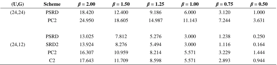
Table 1. Values of TETUE for m= 3 , λ₁ = 1 , λ₂ = 4 , λ₃ = 7 for certain values of (U G, ) and β

(U,G) Scheme β = 2.00 β = 1.50 β = 1.25 β = 1.00 β = 0.75 β = 0.50

(24,24) PSRD 18.420 12.400 9.186 6.000 3.120 1.000

PC2 24.950 18.605 14.987 11.143 7.244 3.631

PSRD 13.025 7.812 5.276 3.000 1.238 0.250

(24,12) SRD2 13.924 8.276 5.494 3.000 1.116 0.164

PC2 16.307 10.959 8.214 5.571 3.229 1.444

C2 17.643 11.709 8.598 5.571 2.893 0.944

Table 2. Values of TETUE for m= 3 , λ₁ = 0.5 , λ₂ = 2.5 , λ₃ = 4.5 for certain values of (U G, ) and β

(U,G) Scheme β = 2.00 β = 1.50 β = 1.25 β = 1.00 β = 0.75 β = 0.50

(24,24) PSRD 23.300 16.964 13.379 9.600 5.840 2.560

PC2 33.454 27.818 24.530 20.978 17.338 14.113

PSRD 16.475 10.687 7.684 4.800 2.317 0.640

(24,12) SRD2 17.612 11.321 8.002 4.800 2.089 0.419

PC2 21.865 16.385 13.444 10.489 7.730 5.613

C2 23.656 17.508 14.074 10.489 6.925 3.668

Table 3. Values of TETUE for m= 4 , λ₁ = 0.25 , λ₂ = 0.5 , λ₃ = 0.75,λ=1.00 for certain values of (U G, ) and β

(U,G) Scheme β = 2.00 β = 1.50 β = 1.25 β = 1.00 β = 0.75 β = 0.50

(24,24) PSRD 53.808 47.050 42.958 38.400 33.688 30.720

PC2 64.252 58.216 54.397 50.000 45.368 43.036

PSRD 38.048 29.639 24.673 19.200 13.369 7.680

(24,12) SRD2 40.674 31.397 25.695 19.200 12.053 5.027

PC2 41.877 34.225 29.779 25.000 20.247 17.083

C2 45.010 36.353 31.041 25.000 18.350 11.727

Table 4. Values of TETUE for m= 6 , λ₁ = 0.03 , λ₂ = 0.06 , λ₃ = 0.09 , λ₄ = 0.12 ,λ₅ =0.15, λ₆ = 0.18 for certain

values of (U G, ) and β

(U,G) Scheme β = 2.00 β = 1.50 β = 1.25 β = 1.00 β = 0.75 β = 0.50

(24,24) PSRD 160.782 176.889 194.097 228.571 317.460 725.624

PC2 197.429 228.982 261.498 326.667 502.331 1443.76

PSRD 113.690 111.433 111.479 114.286 125.984 181.406

(24,12) SRD2 121.537 118.046 116.097 114.286 115.585 118.731

PC2 129.032 134.964 143.445 163.333 222.507 552.366

Proof. See [1]. □ Lemma 4.1. Under PSRD the TETUE equals,

0 :

=1

= ( 1) ( )

G

r r G

r

m R E t

τ

∑

+

Where

1 1

: ,

=1

=1

1 1

( ) = ( ) ( )

r r

r G i r m

i

i j j

c

E t a β

β β− _{γ λ}

Γ

∑

∑

. □ (10)

We now consider PC2 with β_i equal to β . There are m separate experiments, and each experiment lasts until we observe G₀ failures. Let _:

0 ( = 1, , ) r G

t r … m be the time for which the _rth _{experiment lasts.} Clearly, _:

0 ( _{r G} )

E t is obtained from (10) by replacing G

by G₀ and m = 1. We obtain:

Corollary 4.1. Under PC2, for the _ith _experiment ( = 1,i …,m), we have

1 1

: ₀ ,

=1

1 1

( ) = ( ) ( )

r r

r G i r

i i r

c

E t a β

β β γ λ

−

Γ

∑

. □ (11)

To compare the TETUE under PSRD and PC2, we use (10) and (11). We have:

Corollary 4.2. Consider the PSRD and PC2, with β_i 's equal to β . Then the total expected time under the two designs are respectively T₁ and T₂ with

1 :

= 0

= ( 1) ( ),

G

i i G

i

T m

∑

R + E t

0

2 : ₀

=1 =1

= [ ( 1) ( )],

G m

ij ij G i j

T

∑ ∑

R + E t

Where R_ij denotes the number of censored

machines of type i at time t_ij. Theorem 4.2.

i) When U =G , the following result holds:

( )

1

( )

1

1 0

1

=1 1

= (1 )( )

m

m i

i i

i

m

i i

x T mG x e dx

mG β for W eibull

λ θ λ θ

λ β ∞

= =

−

− ′ =

Γ +

∑

∑

∫

∑

ii) For the case of exponential distribution, i.e. when = 1

β and for all U ≥ G, we have

1 2

1 1

, ,

1

m m

i

i i i

mG G G G

T T

m

λ λ

λ

λ

= =

= = = =

∑

∑

where λ and λ are respectively the Arithmetic and the

Harmonic mean of λ_i . Since λ λ≥ , then T₁ ≤T₂.

5. Discussion of Tables

Total expected time under experiment (TETUE) is a very important factor in the composition of the total cost of a test procedure. We will analyze and compare the values of each one of TETUE's associated with the testing procedure and the value of β which has the most effect on the behavior of the hazard function. The following tables involve five kinds of parameters,

, ' ,s m u,

β λ and G . The range of β considered is between 0.5 and 2. Values of λ's are selected in a rather large range (viz. 0.03 to 7.00) so as to cover almost all practical situations. Four sets of values of

's

λ are selected in this range. These four sets respectively correspond to the four tables (1 to 4), the four tables correspond respectively to m=3, 3, 4 and 6, the case m=3 being repeated twice so as to offer a comparison between two sets of values of λ with the same m. Also, in each table, two sets of values of U and G are considered; in one of these sets, we have U=G, and in the second U=2G, so as to provide a common value for all tables, and since G must be divisible by m, we take G=12. In [9], a numerical study of the TETUE was made for SRD2 and C2. For this purpose four sets of values of m,λ′s and β 's were selected. These values are displayed below:

(I) m = 3 λ= (1, 4, 7) ' (II) m = 3 λ= (0.5, 2.5, 4.5 ) '

(III) m = 4 λ= (0.25, 0.5, 0.75, 1.00 ) '

(IV) m = 6 λ= (0.03, 0.06, 0.09, 0.12, 0.15, 0.18 ) ' For each of these sets of values of m and λ, the following values of U G, and β 's were tried:

β = 2.00, 1.75, 1.50, 1.00, 0.75, 050 (U G, ) = (24, 24), (24,12)

We are using the same sets of values of the above parameters for the study of PSRD and PC2.

Consider now T₁ and T₂. It is seen that the values of 1

we use the most common classification of Weibull distribution which is based on the effect of the value β on the hazard function behavior.

The Weibull failure rate for 0< <β 1 is unbounded at 0t = . The failure rate Λ( )t , decreases , thereafter monotonically and is convex, approaching the value of zero as t → ∞, or Λ( )t =0. This behavior makes it suitable for representing the failure rate of units exhibiting early-type failures, for which the failure rate decreases with age. When such behavior is seen, the following reasons can be considered.

•Burn-in testing and/or environmental stress screening are not well implemented.

•There are problems in the production line.

•Inadequate quality control.

•Packaging and transit problems.

It is clear that when 0< <β 1 , the design SRD is better than PSRD and PSRD is better than PC2, in terms of TETUE.

For 1β = , ( )Λ t yields a constant value. This makes it suitable for representing the failure rate of chance-type failure and the useful life period failure rate of machines. In this case PSRD is the same as SRD but it is better than PC2 in terms of TETUE.

For 1,β > Λ( )t increases as t increases and becomes suitable for representing the failure rate of machines exhibiting wear-out type failures. For 1< <β 2 the Λ( )t curve, is concave, consequently, the failure rate increases at a decreasing rate as t increases . For β =2, or the Rayleigh distribution case, there is a

straight line relationship between Λ( )t and t , which goes through the origin with a slop of 2. Λ( )t increases at a constant rate as t increases.

In this case we have that PSRD is the best among all four designs (PSRD, SRD, PC2, C2) in terms of TETUE.

Acknowledgment

We thank the referees for suggesting some changes which led to an improvement in the presentation of this paper.

References

1. Balakrishnan N. and Aggarwala R. Progressive

Censoring: Theory, Methods and Applications.

Birkhauser, Boston (2000).

2. Cox D.R. Partial likelihood. Biometrika, 62: 269-276 (1975).

3. Efron B. The efficiency of Cox’s likelihood function for censored data. J. Amer. Statist. Assoc., 72: 555-565 (1977).

4. Epstein B. Truncated life-test in the exponential case.

Ann. Math. Statist., 25: 555-564 (1954).

5. Epstein B. Estimation from life-test data. Technometric,

2: 447-454 (1960).

6. Khodadadi A. Studies on a general distribution, and testing procedures in life testing. Ph.D. Dissertation, Colorada State University (1990).

7. Murthy D.N.P., M. Xie, and J. Renyan. Weibull Models. John Wiley & Sons, Inc. (2005).

8. Srivastava J.N. Experimental design for the assessment of reliability. In: Basu A.P. (Ed.), Proceeding of the International Symposium on Reliability and Quality Control. North-Holland, Amsterdam (1985).

9. Srivastava J.N. More efficient and less time-consuming censoring designs for life testing. J. Statist. Plann. Inference, 16: 389-413 (1987).

10. Srivastava J.N. and Khodadadi A. Studies on modified and censoring of Type I for comparative experiments under the proportional hazards model. (Unpublished) (1991).

11. Srivastava J.N. Some basic contributions to the theory of comparative life testing experiments. In: Basu A.P. (Ed.),

Advances in Reliability, Elsevier (1993).

12. Zheng G. and Park S. A note on time saving in censored life testing. J. Statist. Plann. Inference, 124: 289-300 (2001).

13. Zheng G. and Park S. Another look at life testing. ibid.,