THERMAL DEVELOPMENT FOR DUCTS OF ARBITRARY
CROSS-SECTIONS BY BOUNDARY-FITTED COORDINATE
TRANSFORMATION METHOD
M. A. Isazadeh
Department of Chemical Engineering, University of Petroleum Industry Ahwaz, Iran
(Received: April 30, 2001 - Accepted in Revised Form: July 20, 2002)
Abstract The non-orthogonal boundary-fitted coordinate transformation method is applied to the solution of steady three-dimensional momentum and energy equations in laminar flow to obtain temperature field and Nusselt numbers in the thermal entry region of straight ducts of different cross-sectional geometries. The conservation equations originally written in Cartesian coordinates are parabolized in the axial direction and then transformed to the non-orthogonal curvilinear coordinate system to handle arbitrary duct geometries. The transformed equations are discretized using the control-volume finite-difference approach in which the convective and diffusive terms are discretized by the upwind and central difference schemes respectively. The discretization equations are solved by a line-by-line TDMA algorithm. Numerical results of Nusselt numbers and temperature profiles are obtained for constant wall temperature boundary condition and Pr = 6.78.
Key Words Boundary-Fitted Coordinates, Thermal Development, Arbitrary Cross-Sectional Ducts
ﻩﺪﻴﻜﭼ
ﻩﺪﻴﻜﭼ
ﻩﺪﻴﻜﭼ
ﻩﺪﻴﻜﭼ
ﺘﻨﻤﻣ ﻱﺪﻌﺑﻪﺳﻲﻤﺋﺍﺩﺕﻻﺩﺎﻌﻣﻞﺣﻱﺍﺮﺑﻲﺳﺪﻨﻫ ﻝﺎﻜﺷﺍ ﺩﻭﺪﺣ ﻩﺪﻧﺮﻴﮔﺮﺑﺭﺩﺪﻣﺎﻌﺘﻣ ﺮﻴﻏﺵﻭﺭ
ﻮ
ﻭﻡ
ﺎﺑﻢﻴﻘﺘﺴﻣﻱﺎﻫﺍﺮﺠﻣﻱﺩﻭﺭﻭﻲﺗﺭﺍﺮﺣﻪﻘﻄﻨﻣﺭﺩﺖﻠﺳﺎﻧﺩﺍﺪﻋﺍﻭﺎﻣﺩﻥﺍﺪﻴﻣﺎﺗﻩﺪﺷﻩﺩﺮﺑﺭﺎﻛﻪﺑﻡﺍﺭﺁﻥﺎﻳﺮﺟﺭﺩﻱﮊﺮﻧﺍ
ﺪﻳﺁﺖﺳﺪﺑﻒﻠﺘﺨﻣﻊﻄﻘﻣﺢﻄﺳ
.
ﺭﺎﻛﺕﺎﺼﺘﺨﻣ ﺭﺩﺍﺪﺘﺑﺍﺭﺩﻪﻛﺎﻘﺑ ﺕﻻﺩﺎﻌﻣ
ﻱﺭﻮﺤﻣﺖﻬﺟﺭﺩ،ﻩﺪﺷﻪﺘﺷﻮﻧ ﻦﻳﺰﺗ
ﻲﻨﺤﻨﻣﺪﻣﺎﻌﺘﻣﺮﻴﻏﺕﺎﺼﺘﺨﻣﻢﺘﺴﻴﺳﻪﺑﺲﭙﺳﻭﻩﺪﺷﻩﺰﻴﻟﻮﺑﺍﺭﺎﭘ
_
ﻲﻣﻝﺎﻘﺘﻧﺍﻲﻄﺧ
ﻩﺍﻮﺨﻟﺩﻲﺳﺪﻨﻫﻝﺎﻜﺷﺍﺎﺗﺪﻨﺑﺎﻳ
ﺪﻧﺮﻴﮕﺑﺍﺭ
.
ﻞﺿﺎﻔﺗﺵﻭﺭﺎﺑﻪﺘﻓﺎﻳﻝﺎﻘﺘﻧﺍﺕﻻﺩﺎﻌﻣ
ﻲﻳﺎﺠﺑﺎﺟﺕﻼﻤﺟﻪﺑﻥﺁﺭﺩﻪﻛﻪﺘﻓﺎﻳﻪﺘﺴﺴﮔﻊﻳﺯﻮﺗ ،ﻲﻫﺎﻨﺘﻣﻱﺎﻫ
ﺵﻭﺭﺎﺑﺐﻴﺗﺮﺗ ﻪﺑﺫﻮﻔﻧﻭ upwind
ﺵﻭﺭﻭ central difference
ﻲﻣﺩﺭﻮﺧﺮﺑ
ﺪﻧﻮﺷ
.
ﻪﺘﺴﺴﮔﻊﻳﺯﻮﺗﻪﻛﻲﺗﻻﺩﺎﻌﻣ
ﻪﺘﻓﺎﻳ ﺪﻧﺍ ،
ﻢﺘﻳﺭﻮﮕﻟﺍ ﺎﺑ TDMA
ﻲﻣﻞﺣ ﻂﺧ ﻪﺑ ﻂﺧ
ﺪﻧﻮﺷ
.
ﻞﻴﻓﻭﺮﭘ ﻭﺖﻠﺳﺎﻧ ﺩﺍﺪﻋﺍﻱﺩﺪﻋ ﺞﻳﺎﺘﻧ
ﻱﺍﺮﺑ ﺎﻣﺩﻱﺎﻫ
ﻩﺭﺍﻮﻳﺩﺖﺑﺎﺛﻱﺎﻣﺩﻱﺯﺮﻣﻂﻳﺍﺮﺷ
٧٨
/
٦
=
Pr
ﺖﺳﺍﻩﺪﺷﻩﺩﺭﻭﺁﺖﺳﺪﺑ
.
1. INTRODUCTION
A review of literature reveals that the majority of the studies in this area were related to rectangular and square ducts. Clark and Kays [1] obtained the fully developed theoretical and experimental Nusselt numbers and temperature profiles for laminar flow constant temperature and constant heat flux boundary conditions in rectangular ducts. Han [2] obtained an analytical solution for fully developed temperature profiles in laminar flow for rectangular ducts with two opposite walls treated as extended surfaces. Sparrow and Siegel [3] obtained the fully developed temperature profiles for constant peripheral heat flux using a variational method. Dennis et al. [4] considered the thermal entrance region problem
Results have been obtained for several duct aspect ratios in the thermal entrance and in the fully developed regions. Neti and Eichhorn [9] presented results of a finite difference study of combined entrance region development (hydrodynamic plus thermal) in square ducts. Temperature profiles and Nusselt number variations are presented for the constant wall temperature case and Pr = 6.0. They have shown that Nusselt number values are smallest near the corners and largest on the central planes.
The objective of the present study is to develop a numerical method by non-orthogoanl boundary-fitted transformation to analyze the thermal entry region of ducts of complex geometry cross-sections [10]. Results are presented for square, triangular, trapezoidal and pentagonal ducts.
2. THE MATHEMATICAL MODELLING
The basic equations, boundary conditions and
simplifying arrangements used in this study
are illustrated in the following sections and
Figures 1 to 6.
The Governing Equations
The strongly conservative form [11] of the steady overall continuity, momentum and energy equations are expressed as follows:The Overall Continuity Equation
(
∇
⋅
ρ
v
)
=
0
(1)The Momentum Equation
(
∇
⋅
ρ
vv
)
−
∇
P
−
( )
∇
⋅
τ
+
ρ
g
=
0
−
(2)The Energy Equation
(
∇
⋅
ρ
C
pTv
)
+
( ) ( )
∇
.
q
+
τ
∇
v
=
0
(3)The conservative form enhances the subsequent treatment of the equations for numerical solution. The body force i.e. the gravitational field is applied only in the “y” direction for the coordinate system selected in Figure 1. For the case where there is a variation of density with temperature in the flow field, the body force term can be modified to a buoyancy force term along with a modified definition of the pressure [12,13]. The buoyant force is the cause of a natural convection flow in the transverse direction.
The Parabolized Governing Equations in
Cartesian Coordinates
The Overall Continuity Equation
0
z
)
w
(
y
)
v
(
x
)
u
(
=
∂
ρ
∂
+
∂
ρ
∂
+
∂
ρ
∂
(4)
The Momentum Equations
x-component
) y x
( x P
) wu ( z ) vu ( y ) u ( x
yx xx
2
∂ τ ∂ + ∂ τ ∂ − ∂ ∂ −
= ρ ∂
∂ + ρ ∂
∂ + ρ ∂
∂
(5)
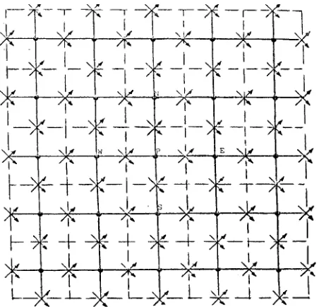
Figure 2. Grid arrangement adopted at each axial section.
y-component
g
)
(
)
y
x
(
y
P
)
pwv
(
z
)
pv
(
y
)
puv
(
x
a yy xy 2ρ
−
ρ
−
∂
τ
∂
+
∂
τ
∂
−
∂
∂
−
=
∂
∂
+
∂
∂
+
∂
∂
(6) z-component ) y x ( dz P d ) pw ( z ) pvw ( y ) uw ( x yz xz 2 ∂ τ ∂ + ∂ τ ∂ − − = ∂ ∂ + ∂ ∂ + ρ ∂ ∂− (7)
The Energy Equation
v P P P .. ) y T k ( y ) x T k ( x ) Tw C ( z ) Tv C ( y ) Tu C ( x Φ µ + ∂ ∂ ∂ ∂ + ∂ ∂ ∂ ∂ = ρ ∂ ∂ + ρ ∂ ∂ + ρ ∂ ∂ (8)
The pressure, P in the above equations is dynamic pressure due to the introduction of buoyancy terms in the “y” momentum equation. In cases of negligible buoyancy effect, P would be the total pressure defined as hydrostatic plus dynamic pressures.
The Boundary Conditions
Inlet (@z = 0)
1. Axial Velocity A uniform entrance velocity profile is specified at inlet:
inlet
w
w
=
(9)2. Transverse Velocities It is assumed that there is no secondary flow at inlet:
u = 0, v = 0 (10)
3. Temperature A uniform temperature profile is assumed at inlet:
wall
T
T
=
(11)Walls of the Duct
1. Axial Velocity No slip-condition is assumed on the walls of the duct:
w = 0 (12)
2. Transverse Velocities
u = 0, v = 0 (13)
3. Temperature For a constant wall temperature:
T = Twall (14)
Outflow Conditions
For the parabolized governing equations used here no downstream boundary conditions are required.3. THE NUMERICAL METHOD OF SOLUTION
The Boundary-Fitted Method
The development of the boundary-fitted method brought about the coordinate transformation of the physical domain, such as Cartesian coordinates to the curvilinearcoordinates so that all the boundaries match the coordinate lines in the new system and the need to interpolate the boundary conditions as practiced before is eliminated [14,15]. The curvilinear coordinate system may be either orthogonal or non-orthogonal in the sense of the mesh generated over the physical-domain. In this study the non-orthogonal method is applied to the solution of the present
dimensional problem arbitrary cross-sectional ducts.
Numerical Grid Generation
This is necessary to determine the location of the coordinate lines in the interior of the physical domain. A coordinate line is specified as being coincident with each boundary line segment while the other coordinate varies monotonically along that line. A method of generating the general boundary-fitted coordinate system is to let the curvilinear coordinates to be the solutions of an elliptic partial differential system in the physical plane, with Dirichlet boundary conditions on all the boundaries.Transformation of Governing PDE’s
It is necessary to transform the partial-differential equations under consideration into the new coordinate variables before being discretized. In general, the transformation operation generates additional terms in the governing equations so that these equations become more complicated upon transformation. The physical Cartesian velocities tire retained as the dependent variables in transformation, however, contravariant velocity components also take part in the structure of the transformed equations. The transformed equations and boundary conditions are as follows:The Overall Continuity Equation
( ) ( ) ( )
U
V
W
=
0
σ
∂
ρ
∂
+
η
∂
ρ
∂
+
ξ
∂
ρ
∂
(15)The Momentum Equations
x-component
( )
( )
[
]
( )
( )
[
yx xx]
[
n n]
yx xx
P
y
P
y
ˆ
y
ˆ
x
ˆ
x
ˆ
y
)
uW
(
)
uV
(
)
uU
(
ξ ξ ξ ξ η η−
−
τ
−
τ
η
∂
∂
−
τ
−
τ
ξ
∂
∂
−
=
ρ
σ
∂
∂
+
ρ
η
∂
∂
+
ρ
ξ
∂
∂
(16) y-component( )
( )
[
]
( )
( )
[
]
[
]
(
)
g
J
P
x
P
x
ˆ
y
ˆ
x
ˆ
x
ˆ
y
)
vW
(
)
vV
(
)
vU
(
a n n xy yy yy xyρ
−
ρ
−
−
−
τ
−
τ
η
∂
∂
−
τ
−
τ
ξ
∂
∂
−
=
ρ
σ
∂
∂
+
ρ
η
∂
∂
+
ρ
ξ
∂
∂
ξ ξ ξ ξ η η (17) z-component( )
( )
[
]
( )
( )
[
]
(
)
g
J
d
P
d
J
ˆ
y
ˆ
x
ˆ
x
ˆ
y
)
wW
(
)
wV
(
)
wU
(
a xz yz yz xzρ
−
ρ
−
σ
−
τ
−
τ
η
∂
∂
−
τ
−
τ
ξ
∂
∂
−
=
ρ
σ
∂
∂
+
ρ
η
∂
∂
+
ρ
ξ
∂
∂
ξ ξ η η (18)The Energy Equation
v P P P
ˆ
ˆ
J
kT
J
kT
J
kT
J
kT
J
)
TW
C
(
z
)
TV
C
(
)
TU
C
(
Φ
µ
+
γ
−
β
η
∂
∂
+
α
−
β
ξ
∂
∂
=
ρ
∂
∂
+
ρ
η
∂
∂
+
ρ
ξ
∂
∂
ξ η η ξ (19)The Boundary Conditions
Inlet (@z = 0)
1. Axial Velocity
( )
,
w
inletw
ξ
η
=
(20)2. Transverse Velocities
( )
,
0
,
v
( )
,
0
3. Temperature
( )
,
T
inletT
ξ
η
=
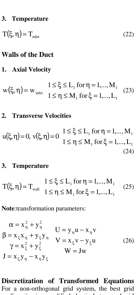
(22)Walls of the Duct
1. Axial Velocity
( )
,
w
inletw
ξ
η
=
1 1 1 1
L
,...,
1
for
M
1
M
,...,
1
for
L
1
=
ξ
≤
η
≤
=
η
≤
ξ
≤
(23)2. Transverse Velocities
( )
,
0
,
v
( )
,
0
u
ξ
η
=
ξ
η
=
1 1 1 1
L
,...,
1
for
M
1
M
,...,
1
for
L
1
=
ξ
≤
η
≤
=
η
≤
ξ
≤
(24) 3. Temperature( )
,
T
wallT
ξ
η
=
1 1 1 1
L
,...,
1
for
M
1
M
,...,
1
for
L
1
=
ξ
≤
η
≤
=
η
≤
ξ
≤
(25)Note:transformation parameters:
ξ η η ξ ξ ξ η ξ η ξ η η
−
=
+
=
γ
+
=
β
+
=
α
y
x
y
x
J
y
x
y
y
x
x
y
x
2 2 2 2Jw
W
u
y
v
x
V
v
x
u
y
U
=
−
=
−
=
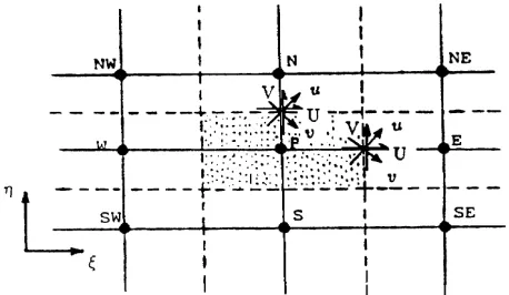
ξ ξ η η (26)Discretization of Transformed Equations
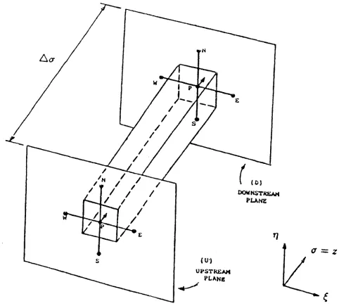
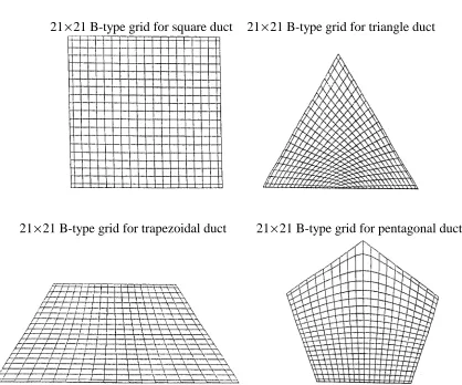
For a non-orthogonal grid system, the best grid configuration is a modified classical staggered-grid in which both components of “if and “v” velocities are used coincidentally at the same location with the contravariant-velocities normal and parallel to the faces of the cell (Figure 2). Physical velocities over the whole computational domain is shown in Figure 3. A three-dimensional control volume is shown in Figure 4.The transformed governing equations are discretized using the method known as the “control-volume” approach [16,17]. The upwind difference scheme is used for discretization of convective terms and the central difference scheme is used for discretization
of diffusion terms. The discretization equations are algebraic equations and are solved by a line-by-line tridiagonal matrix (TDMA) algorithm. For the proper location of the control-volume faces, the B-type grid [17] is employed here. The pressure-velocity coupling in the transverse direction is handled by the SIMPLER algorithm [17] after being modified for the non-orthogonal coordinate system. The method adopted in this work to handle the pressure-velocity coupling in the axial direction is that of Raithby and Schneider [18].
Solution Procedure This work demonstrates the suitability of the numerical model and the solution procedure applied to 3D parabolized momentum and energy equations in straight ducts of arbitrary but uniform cross-sections. A review of some of the related developments in the numerical methods for the solution of conservation equations reveals the elegant features of the numerical procedure applied to this work. In general, coupling between the momentum and mass conservation equations is often the major cause of the slow convergence of the iterative solution methods. Caretto et al. [19] applied a numerical method to the solution of the momentum equations, which involved an implicit simultaneous solution of coupled nonlinear difference equations without linearization or decoupling. The solution procedure was, however, a point-by-point iterative method due to which slow convergence is inevitable. The method of Patankar and Spalding [16] involved linearization and decoupling of the equations. In their method, the non-linear terms (the product terms) of the momentum equations are handled by setting the value of velocities in these terms the same as their values at the previous axial step.
SIMPLE and SIMPLER algorithms [17]. The SIMPLE and SIMPLER algorithms have been already applied to solve problems using the
non-orthogonal boundary fitted coordinate transformation system. Some of these works are worthy to mention here. Hadjisophocleous et al. [21], Shyy et Square Equilateral-triangular Trapezoidal Pentagonal
Figure 5
.
The selected geometries in the physical domain.
21
×
21 B-type grid for square duct 21
×
21 B-type grid for triangle duct
21
×
21 B-type grid for trapezoidal duct 21
×
21 B-type grid for pentagonal duct
al. [22] and Braaten et al. [23] employed the SIMPLE algorithm in their analysis for non-orthogonal systems. Maliska [24] applied a mixed scheme comprising of SIMPLE and SIMPLER algorithms.
The use of nonorthogonal coordinates versus orthogonal system has the advantage of getting rid of the generation of orthogonal grids at certain locations, which are difficult or impossible to make. The staggered grid employed in this work uses both of the u and v velocity components at each velocity locations. This grid arrangement together with the numerical scheme in which both of the physical Cartesian and contravariant velocities are involved, have led the finite difference equations to converge faster without numerical instabilities. Besides, a combination of upwind difference scheme for the convective terms and central difference scheme for the diffusive terms, which is employed in this work, provided satisfactory results.
4. RESULTS AND DISCUSSION
The numerical results of heat transfer analysis for constant wall temperature and Pr = 6.78 are shown
in Figures 7 to 8 and Tables 6 and 7. A general-purpose computer program in Fortran developed by the author was employed to obtain the present results. The specific geometries selected for the present analysis are as flows:
• square duct,
• equilateral triangular duct,
• trapezoidal duct (acute-angle = 60o, one side twice the other),
• pentagonal duct (each angle = 108o). These geometries are shown in Figure 5.
The grids are shown in Figure 6. All the above ducts were selected on the basis of the same equivalent diameter. Consequently, the same value of relaxation factor was applied to all geometries corresponding to each discretization equation. It is believed that this scheme is valid if the geometries selected do not involve oddity. For a pictorial representation of this concept, one may refer to Bejan [25] for a scale drawing of the duct sizes for
some geometry. Other than the ducts mentioned above, circular and rectangular ducts (of two aspect ratios: 2/1 and 3/2) were also examined for validation of the model and the computer code. The problem was solved for an axial step size of 0.276 m for which 250 marching stations were required in the axial direction to reach to the converged solution. For the sake of numerical accuracy and computational economy the mesh size selected was 21 x 21 over the transversed plane. The memory requirement for computations was 2720 K and the typical CPU time was about 26 minutes for one run on IBM ESA9000 machine (mainframe). The computations were performed for fully developed velocity and developing temperature profiles. Referring to Kays et al. [26] the results obtained in this analysis are well suited for the simultaneously developing velocity and temperature profiles for the respective Prandtl number. The buoyancy effect in this study is negligible due to the close temperatures selected for the fluid at inlet and at wall. About 5 iterations were required to obtain converged solution over each transversed plane. The convergence criteria were set on the residual values defined as follows: i. the residual of the energy equation, that is, the
remainder of this equation when the results are substituted for the enthalpy into this equation. In general
R
=
∑
a
nbϕ
nb+
b
−
a
Pϕ
P and R will be zero when the discretization equation is satisfied [17].ii. the residual of enthalpy values, that is, the difference in enthalpy values between two successive iterations.
Table 1 shows the residual values of energy equation and enthalpy values at the converged solution. The local Nusselt number for constant temperature wall boundary conditions, is expressed in terms of the fluid bulk-temperature-gradient along the flow path length by
* *
b
b T
, z
dZ d 4
1
Nu θ
θ −
= (27)
Refer to the Appendix for derivation.
wall temperature boundary condition is expressed by:
θ
=
b *
* T
, m
1
ln
Z
4
1
Nu
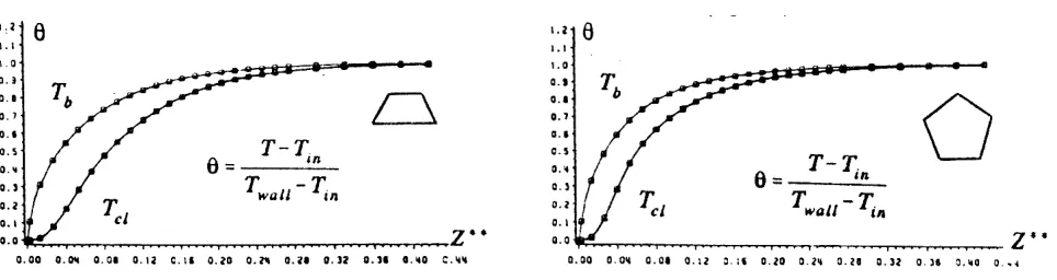
(28)which is obtained from Equation 27by integration. The thermal entry length is analyzed in terms of the dimensionless bulk and centerline temperatures in Figure 7(a, b) and Figure 8(a, b) for square, triangular, trapezoidal and pentagonal ducts. Bulk temperature is the mean temperature over the section and centerline temperate is the mean temperature over the centerline. The thermal entry length obtained in this study for square ducts is
TABLE 1. Residual Values.
Geometry Energy-equation Residual
Enthalpy Residual
Square 0.303
×
10-7 -0.275×
10-4 Triangular 0.160×
10-6 -0.270×
10-4 Trapezoidal 0.533×
10-7 -0.270×
10-4 Pentagonal 0.694×
10-7 -0.385×
10-4 Rectangular(2/1)
0.224
×
10-7 -0.357×
10-4 Rectangular(3/2)
0.262
×
10-7 -0.315×
10-4 Circulare 0.105×
10-6 -0.501×
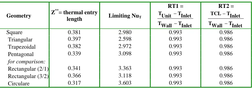
10-4TABLE 2. Thermal Entry Length and Limiting NuT Results.
Geometry Z
**
= thermal entry
length Limiting NuT
RT1 =
Inlet T Wall T
Inlet T Unit T
− −
RT2 =
Inlet T Wall T
Inlet T TCL
− −
Square 0.381 2.980 0.993 0.986
Triangular 0.397 2.598 0.993 0.986
Trapezoidal 0.382 2.972 0.993 0.986
Pentagonal 0.339 3.098 0.993 0.986
for comparison:
Rectangular (2/1) 0.341 3.363 0.993 0.986
Rectangular (3/2) 0.366 3.118 0.993 0.986
Circulare 0.317 3.603 0.993 0.986
TABLE 3. Comparison of Limiting Nusselt Numbers.
Square Rectangular (2/1)
Rectangular (3/2)
Equilateral
Triangular Circular
Clark and Kays 2.890 3.390 - - -
Dennis et al. 2.980 3.390 3.120 - -
Shah and London 2.976 3.391 3.117 - -
Schmidt 2.970 3.383 3.121 - -
Javeri 2.981 3.393 - - -
Lyczkowski et al. 2.975 3.395 3.117 - -
Kays and Crawford 2.980 3.390 - 2.350 3.658
Wibulswas - - - 2.570 -
Z** = 0.381 which is close to the value obtained by Neti et al. [9], Z** = 0.352. The value in this study is corresponding, however, to the dimensionless bulk and centerline temperatures of 0.993 and 0.986 respectively while the values obtained by Neti et al. [9] are that of 0.988 and 0.979 respectively. The temperature is nondimensionalized here with the difference between the fluid wall temperature and the fluid temperature at the duct entrance. The results for the limiting Nusselt numbers are indicated in Table 2 for all geometries under consideration. The limiting Nusselt numbers (
Nu
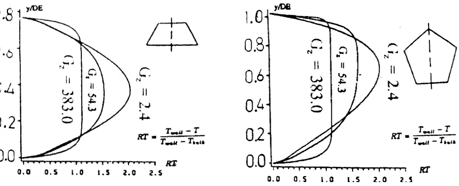
T) for square, rectangular, triangular and circular ducts obtained in this study are compared with the analytical and numerical results of other investigators in Table 3. These results confirm the validity of the model and computer code in this study.The results of central plane thermal development are shown in Figures 9(a, b) and 10(a, b) for square, triangular, trapezoidal and pentagonal ducts in terms of the dimensionless temperature profiles. The temperature is nondimensionalized here with the difference between the uniform wall temperature and the bulk fluid temperature. Temperature profiles are shown at three different axial positions. The peak value of RT for triangular and pentagonal ducts tends towards the corner of the ducts on the central plane. This is due to zero friction at corners due to which the peak value of velocity profile on the central plane tends closer to
the corner and induces temperature accordingly. The results obtained for square ducts for Newtonian fluids (
Nu
z,T,Nu
m,T) are comparedwith the numerical solutions of Chandrupatla & Sastri [27] in Tables 4 and 5. There is a close agreement between their solutions and the present results for
Nu
z,T but there are some differences betweenNu
m,T values. The results obtained byChandrupatla and Sastri [27] are with no secondary flow and no viscous dissipation effects. Also, the effect t of variation of Prandtl number is ignored in their analysis and no value is mentioned for the Prandtl number corresponding to their results. It is believed that, the differences existing in the results of
Nu
m,T as observed in Table 5 are mainly due to the difference in the values of Prandtl numbers. Chandrupatla and Sastri [27] ignores the effect of Prandtl number onNu
m,T by reasoning that it is included in the relevant( )
X
4
Pr
term. However,
T , m
Nu
is affected by Pr through the effectθ
baccording to the following relations:
( )
θ
=
θ
=
b b
T , m
1
ln
4
X
Pr
4
1
1
ln
X
Pr
Nu
(29)TABLE 4. Comparison of Nusselt Number: Nuz,T Variation for Square Ducts.
Chandrupatla Present Analysis
Gz Nuz,T Gz Nuz,T
0 2.975 0 2.980 40 3.432 37 3.204 50 3.611 50 3.527 80 4.084 75 4.104 100 4.357 100 4.635 133.3 4.755 127 4.845
200 5.412 190 5.808
TABLE 5. Comparison of Nusselt Number: Num,T Variation for Square Ducts.
Chandrupatla Present Analysis
Gz Nuz,T Gz Nuz,T
0 2.975 0 2.980 40 4.841 37 4.878 50 5.173 50 5.441 80 5.989 75 6.386 100 6.435 100 7.186 133.3 7.068 127 8.084
or
θ
=
b z T
, m
1
ln
G
4
1
Nu
(30)but
( )
Pr
f
b
=
θ
(31)therefore
( )
Pr
g
G
4
1
Nu
m,T=
z (32)or
(
G
,
Pr
)
h
Nu
m,T=
z (33)The results of local and mean Nusselt numbers for ducts of different cross-sectional geometries are presented in Tables 6 and 7.
5. CONCLUSIONS
This paper shows the application of a non-orthogonal boundary fitted coordinate (BFC) procedure in the solution of 3D parabolized momentum and energy equations for various non-circular cross-sectional ducts. The thermal entrance region temperature profiles, thermal entry lengths, Nusselt number variations and limiting Nusselt number values are obtained for square, triangular, trapezoidal and pentagonal ducts. Experimental work is required in the entrance region of noncircular ducts to verify some of the results.
Figure 7. (a, b) D. L. temperature vs. D. L. axial distance, (square, triangular).
6. NOMENCLATURE
a coefficient in the discretization equations AR aspect ratio
b constant term in the discretization equations Cp specific heat
D. L. dimensionless
Dh, DE hydraulic diameter (or equivalent diameter)
DE = 4rh =
perimeter
wetted
area
flow
4
×
g acceleration due to gravity Gz Greatz number ( z **
Z
1
G
=
) h enthalpy (h = CPT)I index of “
ξ
” axis in transformed plane J index of “η
” axis in transformed plane J Jacobian of transformationk thermal conductivity
L1 maximum value of “I” index (on “
ξ
” axis) M1 maximum value of “J” index (on “η
” axis) Nuz,T local Nusselt numberNum,T mean Nusselt number
NuT limiting Nusselt number
P total pressure (dynamic + hydrostatic) P dynamic pressure
P
mean viscous pressure Pr Prandtl number (Pr =k
C
Pµ
)
Pe Peclet number (Pe = Re . Pr =
k
w
D
C
P hρ
)
q heat flux
R residual of discretization equation Re Reynolds number (Re =
( )
µ
ρ
D
hw
) T temperature
TABLE 6. Nuz,T, Variations of Different Geometries.
Gx Square Triangular Trapezoidal Pentagonal
100 4.635 4.373 4.564 4.689
75 4.104 3.871 4.025 4.157
60 3.767 3.575 3.701 3.844
50 3.527 3.377 3.479 3.633
43 3.345 3.234 3.314 3.481
37 3.204 3.126 3.186 3.366
0 2.980 2.598 2.979 3.098
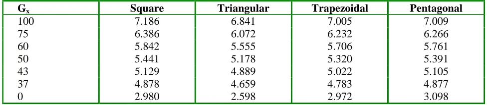
TABLE 7. Num,T Variations of Different Geometries.
Gx Square Triangular Trapezoidal Pentagonal
100 7.186 6.841 7.005 7.009
75 6.386 6.072 6.232 6.266
60 5.842 5.555 5.706 5.761
50 5.441 5.178 5.320 5.391
43 5.129 4.889 5.022 5.105
37 4.878 4.659 4.783 4.877
tl inlet temperature
tw wall temperature
u, v, w velocity components in the Cartesian system U, V, W contravariant velocity components [v] average axial velocity coefficients v velocity field
w
mean axial velocityx, y, z Cartesian coordinate system X dimensionless axial distance Z** dimensionless axial-distance, Z** =
e h
P
D
z
Figure 9. (a, b) Development of the temperature profile, (square, triangular).
Greek Letters
γ
β
α
,
,
transformation coefficientsσ
η
ξ
,
,
axes of curvilinear coordinateµ
viscosityρ
densitya
ρ
arithmetic mean densityv
φ
viscous dissipation functionij
τ
stress-tensorij
∆
rate of deformation tensorθ dimensionless temperature,
w l w
t
t
t
t
−
−
=
θ
φ
a general dependent variableSubscripts
nb general neighbor grid point
Superscripts
^ refers to the transformed quantity
7. APPENDIX
Derivation of Local and Mean Nusselt Number
From Bird [11] (Page 423):
(
) (
)
(
w b)
loc b o locT
T
Pdz
h
dQ
T
T
Ddz
h
dQ
−
=
→
−
=
π
(34) in which P: perimeter, To = Tw = Twall[ ]
b P c b PdT
w
C
A
dQ
dT
v
C
D
dQ
ρ
ρ
π
=
→
=
4
2 (35) in which Ac cross-sectional area(
)
(
)
dz T T dT w C P A h b w b P cloc −
= µ ρ
µ (36)
( )
( )
(
T T)
dz dT DE w k C P A k DE h Nu b w b P c loc loc − = = µ ρ µ (37)( ) ( ) (
T
T
)
dz
dT
P
A
Nu
b w b c loc−
=
Pr
Re
(38)(
)
(
)
(
) (
DE
Re
Pr
)
dz
1
T
T
T
T
T
T
dT
P
DE
A
Nu
l w b w l w b c loc⋅
⋅
−
−
−
⋅
=
(39)(
)
l w b w l w bT
T
T
T
d
T
T
dT
−
−
−
=
−
b l w b wd
T
T
T
T
d
=
−
θ
−
−
−
=
(40)
in which l w b w bT
T
T
T
−
−
=
also
* *
dZ
Pe
DE
z
d
Pr
Re
DE
dz
=
⋅
=
⋅
⋅
(42)and from the definition DE = 4 P A
one can write
4 1 P DE
Ac =
⋅
therefore
* *
b
b loc
dZ d 4
1
Nu θ
θ −
= (43)
∫
∫
⋅
=
−
θbθ
θ
* *
1 b
b *
* Z
0 loc
d
4
1
Z
d
Nu
(44)b *
* T ,
m
ln
4
1
Z
Nu
⋅
=
−
θ
(45)8. REFERENCES
1. Clark S. H. and Kays, W. N., “Laminar Flow Forced Convection in Rectangular Ducts”, Trans. ASME 75, (1953), 859-866.
2. Han, L. S., “Laminar Heat Transfer in Rectangular Channels”, J. Heat Transfer, Trans. ASME Series C81, (1959), 121-128.
3. Sparrow M. and Siegel, R., “A Variational Method for Fully Developed Laminar Heat Transfer in Ducts”, J. Heat Transfer, Trans. ASME Series C81, (1959), 157-167. 4. Dennis, S. C. R., Mercer, A. McD. and Poots, G.,
“Forced Heat Convection in Laminar Flow through Rectangular Ducts”, Quart. Journal Appl. Math., Vol. 17, (1959), 285-297.
5. Savino, J. M. and Siegel, R., “Laminar Forced Convection in Rectangular Channels with Unequal Heat
Addition on Adjacent Sides”, Int. Journal Heat Mass Transfer, Vol. 7, (1964), 733-741.
6. Montgomery, S. R. and Wibulswas, P., “Laminar Flow Heat Transfer in Ducts of Rectangular Cross-Section”,
ibid., Vol. 1, (1966).
7. Shah, R. K. and London, A. L., “Laminar Flow Forced Convection in Ducts”, Academic Press, New York, (1978).
8. Lyczkowski, R. W., Solbrig, C. W. and Gidaspow, D., “Forced Convection Heat Transfer in Rectangular Ducts”, Nucl. Eng. and Design, Vol. 67, (1981), 357-378.
9. Neti, S. and Eicbhorn, R., “Combined Hydrodynamic and Thermal Development in a Square Duct”, Num. Heat Transfer, Vol. 6, (1983), 497-510.
10. Isazadeh, M. A., “Numerical Solution of Reacting Laminar Flow Heat and Mass Transfer in Ducts of Arbitrary Cross-Sections for Power-Law Fluid”, Ph.D Thesis, McGill University, Montreal, Canada, (1993). 11. Bird, R. B., Steward, W. E. and Lightfoot, E. N.,
“Transport Phenomena”, John Wiley and Sons, N. Y., (1960).
12. Allen, P. H. C., “Heat and Mass Transfer by Combined Forced and Natural Convection”, The Institution of Mechanical Engineers, (1972).
13. Ostrach, S., “Laminar Natural-Convection Flow and Heat Transfer of Fluids with and without Heat Sources in Channels with Constant Wall Temperature”, NACA Technical Note 2863, (1952).
14. Chu, W. H., “Development of a General Finite Difference Approximation for a General Domain”,
Journal Cornp. Physics, Vol. 8, (1971), 392-408. 15. Thompson, J. F., Thames, F. C., and Mastin, C. W.,
“Boundary-Fitted Curvilinear Coordinate Systems for Solution of Partial Differential Equations on Fields Containing any Number of Arbitrary Two-Dimensional Bodies”, Report CR-2729, NASA Langley Research Centre, (1977).
16. Patankar, S. V., and Spalding, D. B., “A Calculation Procedure for Heat, Mass and Momentum Transfer in Three-Dimensional Parabolic Flows”, Int. J. Heat Mass Transfer, Vol. 15, (1972), 1787-1806.
17. Patankar, S. V., “Numerical Heat Transfer and Fluid Flow”, Hemisphere Publishing Corporation, N. Y., (1980).
18. Raithby, C. D. and Schneider, G. E., “Numerical Solution of Problems in Incompressible Fluid Flow: Treatment of the Velocity-Pressure Coupling”,
Numerical Heat Transfer, Vol. 2, (1979), 417-440. 19. Caretto, L. S., Curr, R. M. and Spalding, D. B., Comp.
Meth. Appl. Mech. and Engr., Vol. 1, No. 39, (1973). 20. Briley, W. R., “Numerical Method for Predicting Three
Dimensional Steady Viscous Flow in Ducts”, Journal Comp. Physics, Vol. 14, (1974), 8-28.
21. Hadjisophocleous, G. V., Sousa, A. C. M. and Venart, J. E. S., “Prediction of Transient Natural Convection in Enclosure of Arbitrary Geometry Using a No Orthogonal Numerical Model”, Numerical Heat Transfer, Vol. 13, (1988), 373-392.
Coordinate System”, Numerical Heat Transfer, Vol. 8, (1985), 99-113.
23. Braaten, M. and Shyy, W., “A Study of Recirculating Flow Computation Using Body-Fitted Coordinates: Conszstency Aspects and Mesh Skewness”, Numerical Heat Transfer, Vol. 9, (1988), 559-574.
24. Maliska, C. R. and Raithby, G. D., “A Method for Computing Three-Dimensional Flows Using Non-Orthogonal Boundary-Fitted Coordinates, Int. J. for Numerical Methods in Fluids, Vol. 4, (1984), 519-537. 25. Bejan, A., “Convection Heat Transfer”, Prentice Hall, N.
J., (1984).
26. Kays, W. M. and Crawford, M. E. “Convective Heat and Mass Transfer”, Second Ed., McGraw Hill, N. Y., (1980).
27. Chandrupatla, R. and Sastri, V. M. K., “Laminar Forced Convection Heat Transfer of a Non-Newtonian Fluid in a Square Duct”, Int. Journal Heat Mass Transfer, Vol. 20, (1977), 1315-1324.