A Trust Region Algorithm for Solving Nonlinear Equations (RESEARCH NOTE)

RESEARCH

NOTE

A TRUST REGION ALGORITHM FOR SOLVING

NONLINEAR EQUATIONS

S. J. Sadjadi

Department of Industrial Engineering Iran University of Science and Technology Tehran, Iran [email protected]

(Received: April 27, 2001 – Accepted: October 18, 2001)

Abstract This paper presents a practical and efficient method to solve large-scale nonlinear equations. The global convergence of this new trust region algorithm is verified. The algorithm is then used to solve the nonlinear equations arising in an Expanded Lagrangian Function (ELF). Numerical results for the implementation of some large-scale problems indicate that the algorithm is efficient for these classes of problems.

Key Words Trust Region, Nonlinear Equations, Newton Method

ﻩﺪﻴﻜﭼ

ﻪﻟﺎﻘﻣﻦﻳﺍﺭﺩ

ﺑﺩﺎﻌﺑﺍﺭﺩﻲﻄﺧﺮﻴﻏﺕﻻﺩﺎﻌﻣﻞﺋﺎﺴﻣﻞﺣﻱﺍﺮﺑﻲﻠﻤﻋﻭﺪﻣﺁﺭﺎﻛﺵﻭﺭﻚﻳ ﻪﺋﺍﺭﺍﮒﺭﺰ

ﻲﻣ ﺩﻮﺷ .

ﺎﻧﻞﺣﻱﺍﺮﺑﻢﺘﻳﺭﻮﮕﻟﺍﺲﭙﺳﻭﻩﺪﺷﺕﺎﺒﺛﺍﺩﺎﻤﺘﻋﺍﻪﻴﺣﺎﻧﻢﺘﻳﺭﻮﮕﻟﺍﻦﻳﺍﻲﻳﺍﺮﮕﻤﻫﺍﺪﺘﺑﺍ ﺕﻻﺩﺎﻌﻣ

ﻲﻄﺧﺮﻴﻏ

ﻲﻣﺭﺍﺮﻗﻩﺩﺎﻔﺘﺳﺍﺩﺭﻮﻣﮋﻧﺍﺮﮔﻻﻂﺴﺑﻊﺑﺍﻮﺗﺭﺩ ﺩﺮﻴﮔ

.

ﻳﺭﻮﮕﻟﺍﻦﻳﺍﺯﺍﻩﺩﺎﻔﺘﺳﺍﺎﺑﺕﺎﺒﺳﺎﺤﻣﺞﻳﺎﺘﻧ ﺪﻣﺁﺭﺎﻛﺮﮕﻧﺎﺸﻧﻢﺘ

ﺖﺳﺍﻞﺋﺎﺴﻣﻲﻀﻌﺑﻱﻭﺭﺮﺑﻥﺁﻥﺩﻮﺑ .

1.INTRODUCTION

The use of trust region methods for solving systems of nonlinear equations has been popular during the past decade. Much of the interest is due to the strong convergence properties of such methods [1,2]. Duff et al.[3] use linear programming combined with trust region idea to solve nonlinear equations. It is based on minimizing the l₁-norm of the linearized vector within an

l

_∞norm trust region, thereby permitting linear programming techniques to be easily applied. Duff et al. [3] show that their approach works better than Levenberg's algorithm [4]. However, the algorithm was not used for large-scale problems. Luksan [5] uses an inexact trust region method to solve large and sparse nonlinear equations. The method does not need to use matrices so it can be also used for large dense nonlinear equations. Martinez [6] uses a two-dimensional search algorithm

to solve large and sparse nonlinear equations. Although the algorithm has strong convergence properties, the computation of the two dimensional search is expensive.

Martinez and Santos [7] tried to solve this difficulty by using a curvilinear search algorithm. This paper presents a modification of a trust region algorithm introduced by Martinez [7]. Our algorithm has a curvilinear search method similar to that proposed by Martinez and Santos [7], and our convergence proof eliminates mistakes in their work. Numerical results of a large-scale problem are presented at the end.

2. PROBLEM STATEMENT

n

R xmin_∈

2 ) x ( F 2 1

where F = (f₁,...,f_m)T is a C -function and . 1 represents the Euclidean norm in Rn. Martinez's method [6] uses a Gauss-Newton strategy to obtain an approximation of the Newton direction. Bi-dimensional search methods are then used to find the best direction

d

_k+1, which is a linear combination of the Newton direction and the Cauchy step at every iteration.

The algorithm developed by Martinez [6] needs to solve a bi-dimensional search direction several times. This makes the algorithm inefficient in some cases, especially for large-scale problems. Martinez and Santos [7] present a modification of their method, and report that the use of a curvilinear search method can reduce the burden of the computation and significantly simplify the algorithm for practical implementation. However, the curvilinear search plane used in the algorithm statement by Martinez and Santos is different from what they actually developed. In the following section, we present a new curvilinear search method.

The contributions of the proposed method in addition include the use of a pure Newton direction near optimal solution.

A convergence proof is given at the end that eliminates the mistakes in the work of Martinez and Santos [7].

3. A NEW ALGORITHM WITH CURVILINEAR SEARCH DIRECTION

In this section we present a proposed algorithm that has similar steps as the algorithm in [7]. We consider that a Newton step tends to provide fast convergence when x is close enough to

x

*. Therefore, we switch the bi-dimensional search direction to a pure Newton step when step

d

_k is close enough to the final step.

Algorithm 1

Let

F

:

Ω

⊂

R

n

→

R

m

,

m

≥

n

Ω

Ω

∈

C

(

),

F

1 _{an open set. Let} 0 _∈Ω

x be an

arbitrary initial point,

) 1 ,. 0 [ ), 2 1 , 0 [ ), 1 , 0 [ , ), 1 , 0

[ _{1 2 3}

k ∈ θ θ ∈ θ ∈ ξ∈

η

]. M , M [ M , 0

M_{> ∈ θ1}

Let x be the k-th approximation to the solution. _k We denote

) ,..., ( diag D

, x ) x ( F 2 1

F J g ), x ( J J ), x ( F F

n k 1

k k

k 2

k T k k k k k k

σ σ = ∇

= = =

=

(1)

where

    

> < ∈ =

σ

. M ) x ( if M

, M ) x ( if M

], M , M [ ) x ( if ) x (

2 i k

2 i k 2 i k 2

i k i

k

Step 1 Compute J_kand g_k. If g_k=0, stop.

Step 2 Obtain w_k∈Rn such that .

g g

w J

JT_{k k k + k ≤ηk k} (2)

If g_{k ≤ε} set x_k+1 =x_k +w_kand k=k+1, go to Step 1.

Step 3 Obtain n

k

R

v

∈

as the solution of the following bi-dimensional problem:

k k 2 k 1 k

k

v

F

.s

.t

g

w

w

J

min

+

λ

+

λ

≤

(3)

Step 4 Set d1_{k =−}g_k and test the following two conditions for v_k:

k k 1 k T

kg v g

v _≤−θ (4)

and

k k

k v Mg

g

If (4) and (5) are satisfied set dk₂ =v_kotherwise set k

1 k

2 d

d = .

Step 4 Set t = 1. Perform Step 5.a to 5.d

(5.a): Set d=d (t)= ₁ 2 1_k k

T k

2 k T k 2 k

2 _{t(1 t )d}

d g

d g d

t _{+ −} (6)

(5.b): If F(x ) g d 2

1 ) d x ( F 2

1 T

k 2 2 k 2

k+ ≤ +θ (7)

go to Step 5.d

(5.c): Let

t

ˆ

be such that θ₃d(t) ≤ d(tˆ) ≤(1−θ₃)d(t)

(8) Replace t by

t

ˆ

, go to Step 5.a

(5.d): d_k =d, x_k+1 =x_k +d_k.

Algorithm (1) has similar steps as the one introduced by Martinez [7]. In Step 5.a, we are using a new curvilinear search algorithm, which is slightly different from the original algorithm.

Theorem 1. The Algorithm 1 is well defined. The proof is similar to Martinez and Santos [7] and corrects the mistakes in the original paper.

It is an easy task to show that if

g

k

≠

0

, the algorithm can reach Step 5.d in a finite number of iterations. In Step 2 of the algorithm, a system of linear equations is solved. Assuming that the system of equations has full rank, it always has a unique solution. In Step 3, a two-dimensional sub problem is solved and v is in the positive cone determined by g_kand w_k. Step 4 does not create any problems. Finally, Step 5 is verified as follows. Let us write

, d ) t 1 ( at d t ) t ( d

d= = 2 ₂+ − 2 ₁ where ₁

k T k

2 k T k d g

d g a₌ . By the definition of

d

_k1 and (4) we know that a > 0. By (8), we need to show that (7) is satisfied when t is small enough. By Mean Value Theorem,

) t ( d )) t ( d ) t ( g ( g

) x ( F 2 1 )) t ( d x ( F 2 1

T k

2 k 2

k

ξ + =

− +

(10)

where g(x) denotes F(x)2 2

1

∇ and .0_≤ξ(t)_≤1 Meanwhile, d (t) is a positive combination of

1

d and d in (6), ₂ g_kTd1_k <0and gT_kd2_k <0. Therefore 0

) t ( d

gT_k < for ]t_∈[0,1 . So, by (10)

1 k T k

1 k T k T

k

T k

T k

2 k 2

k 0

t

d ) x ( g

d ) x ( g )

t ( d g

) t ( d )) t ( d ) t ( x ( g

) t ( d g

) x ( F 2 1 )) t ( d x ( F 2 1 lim

= ξ

+

= −

+ →

(11)

Taking limits on both sides of (11), we have

1 d

g

) x ( F 2 1 ) d x ( F 2 1

1 k T k

2 k 2

1 k k

= −

+

(12)

Therefore, given θ₂∈(0,1), there exists ∧t_>0such that

2 T

k

2 k 2

k

) tˆ ( d g

) x ( F 2 1 )) tˆ ( d x ( F 2 1

θ ≥ −

+

(13)

for ).t_∈(0,tˆ Thus, using gT_kd(tˆ)<0, we obtain (7). This completes the proof.

Theorem 2. Assume that (

x

_k) is generated by algorithm 1, Then:

If there exists c > 0 such that g_{k ≤}cfor all k=0,1,2,… and _x*∈Ω _{is a limit point of (x )}

k , then J(x*)TF(x*)=0.

(a) Let ε>0. If x_∈Ω: F(x)2 _≤ F(x0) 2 is compact, then there exists k∈Nsuch that

ε ≤

) x ( F ) x (

J T _k

(b) Let x* be a strict local minimizer of f in 0

,ε≥

Ω . Then there exists ε₁>0such that 1

* k x

x − ≤ε .

(c) If x*is a local minimizer of F(x_k)2and an isolated stationary point in

Ω

, then there exists ε>0such that limx_k =x*, whenever

ε ≤ − * 0 _x

x .

Proof 2 We prove that if the inequality 2

k

k d

d _≤ in (8) is changed to 2 k k Kd

d _≤ for

some constant K, it will become a simple case of the algorithm 3.1 of [6]. It is clear that the Equations 4 and 6 and the definition of d1_k implies that )d C(d ,d2

k 1 k

k ∈ . It can be also verified that

1 k

d satisfies:

k 1 k 1 1 k T

kd d g

g _≤−θ (14)

In fact, 1 k k 2 k k k k k k T k 1 k k 1 k T k M / M g g g M M g D g g D g d g d g θ ≥ = ≥

= (15)

Therefore, (14) is proved. Now, by (4) and (5) and the choice of d2_kwe have:

k 2 k 1 2 k T

kd d g

g ≤ −θ (16)

Hence the axiom (2) of [6] is satisfied. By definition of d , we have: 1_k

k 1

k

k

d

M

g

g

M

≤

≤

(17)

Hence, by (4), (5), the axiom (9) of [6] is also satisfied. On the other hand, by (7), the axiom (9) of [6] holds. Finally, we prove the inequality of

2 k k

K

d

d

≤

. From the Expression 9 for d(t) it

implies that 1

k 2 2

k

a

(

1

3

t

)

d

td

2

)

t

(

d

′

=

+

−

Therefore, if

γ

(

t

)

=

d

(

t

)

2

,

for

t

∈

[

0

,

1

]

, there is

=

−

+

−

+

=

′

=

γ′

)

d

)

t

1

(

at

d

t

(

)

d

)

t

3

1

(

a

td

2

(

2

)

t

(

d

)

t

(

d

2

)

t

(

1 k 2 2 k 2 T 1 k 2 2 k T 2 k T 1 k 2 2 2 k T 1 k 2 2 2 k T 2 k

3_{d d 2at (1 t )d d at (1 3t )d d} t

2 [

2 + − + −

+

a

t

(

1

−

3

t

)(

1

−

t

)

d

d

1

]

=

k T 1 k 2 2 2 2 k T 1 k 2 2 2 2 2 2 k

3

d

[

4

a

(

1

t

)

2

at

(

1

3

t

)]

d

d

t

4

+

−

+

−

+ 1 2

k 2 2

2

t

(

1

3

t

)(

1

t

)

d

a

2

−

−

2 1 k 2 2 k T 1 k 2 2

k

6

ad

d

2

a

d

d

4

+

+

≤

1 k k 1 2 1 k 2 k k 1 k k 1 1 k 1 k 2 k k 2 k 2 d g d d g 2 d g d d d g 6 g M 4 θ + θ + ≤ 1 2 k 2 1 2 k 2 2 k

2

6

M

g

2

M

g

g

M

4

θ

+

θ

+

≤

2 k 1 2 k 1 2 1 2 2

g

C

g

)

M

2

M

6

M

4

(

=

θ

+

θ

+

≤

(19)

Therefore, for

t

∈

[

0

,

1

],

.

d

)

M

C

1

(

M

d

C

d

g

C

d

)

t

(

max

)

1

(

)

t

(

)

t

(

d

2 2 k 2 1 2 2 2 k 1 2 2 k 2 k 1 2 2 k ] 1 , 0 [ t 2

+

=

+

≤

+

≤

γ′

+

γ

≤

γ

=

_∈ .

Thus (18) is satisfied with 1₂

M

C

1

K

=

+

and the proof is complete.

4. MOTIVATION

is explained. Since d(t) lies in the positive cone generated by

d

1_k and

d

2_k for all

t

∈

[

0

,

1

]

and it is desired to have a negative gradient direction when the step is infinitesimal, the search direction is assumed to be tangent to

d

1_k for small step t. (Note that

d

(

1

)

d

,

d

k

(

0

)

0

,

a

0

)

2 k

k

=

=

>

. Let h be the orthogonal projection of

d

2_k on the orthogonal complement of the line generated by

d

1_k, related to the norm

.

(

z

z

D

1

z

k T 2 D

D 1

k 1 k

−

=

−

− for all

z

R

)

n

∈

,

Therefore,

,

d

d

D

d

d

D

d

d

h

1

k 1 k 1 k T 1 k

1 k 1 k T 2 k 2

k ₋

−

−

=

But 1 _{k k}

k

D

g

d

=

−

, hence,

.

d

d

d

d

g

d

h

1

k 1 k T k

2 k T k 2 k

−

=

For each point z in the plane spanned by (

d

1

,

h

k ) may be expressed as

z

=

y

1

d

1k

+

y

2

h

.

2 k

d

corresponds to

,

y

1

d

g

d

g

y

_{1 2}

k T k

2 k T k

1

=

=

. A simple curve proposed by Martinez [7] has the following form:

},

)

y

d

g

d

g

(

y

|

h

y

d

y

z

{

P

2

1 2 k T k

1 k T k 2 2 1 k

1

+

=

=

=

and the curve used by Martinez and Santos, in the coordinate

(

y

₁

,

y

₂

)

has the form:

)}.

y

y

y

(

d

g

d

g

y

|

h

y

d

y

z

{

P

2 2

2 1 k T k

2 k T k

1 2 1 k 1

2 3

+

+

−

=

+

=

=

5. NUMERICAL IMPLEMENTATION AND RESULTS

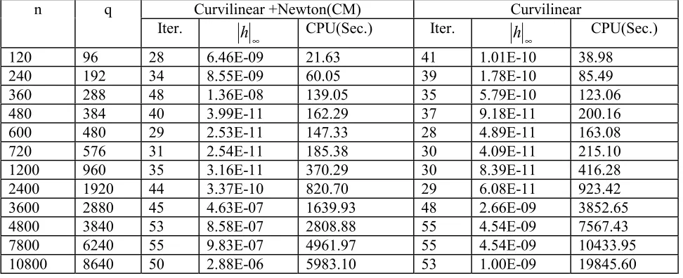
In this section some numerical results for the implementation of the curvilinear search method to solve a large-scale problem from water resources management are presented. The problem has the form of the minimization of a quadratic objective function, f(x), subject to some equality constraints, h(x), and some bound constraints, g(x). The TABLE 1. The Summary of the Use of Algorithm 1.

Curvilinear +Newton(CM) Curvilinear n q

Iter.

∞

h

CPU(Sec.) Iter.

h

_∞ CPU(Sec.)

120 96 28 6.46E-09 21.63 41 1.01E-10 38.98

240 192 34 8.55E-09 60.05 39 1.78E-10 85.49

360 288 48 1.36E-08 139.05 35 5.79E-10 123.06

480 384 40 3.99E-11 162.29 37 9.18E-11 200.16

600 480 29 2.53E-11 147.33 28 4.89E-11 163.08

720 576 31 2.54E-11 185.38 30 4.09E-11 215.10

1200 960 35 3.16E-11 370.29 30 8.39E-11 416.28

2400 1920 44 3.37E-10 820.70 29 6.08E-11 923.42

3600 2880 45 4.63E-07 1639.93 48 2.66E-09 3852.65

4800 3840 53 8.58E-07 2808.88 55 4.54E-09 7567.43

7800 6240 55 9.83E-07 4961.97 55 4.54E-09 10433.95

Expanded Lagrangian Techniques developed in [8] is used to convert the constrained optimization into a set of nonlinear equations in order to use the curvilinear search algorithm developed in this paper.

The implementation uses

5 9

3 4

2 7 1

4_{, 10 , 10 , 10 ,M 10 ,M 10}

10− _{θ =} − _{θ =} − _ξ= − _{= =} −

= η

In Table 1, we report:

(n, q, Iter.): the number of variables, the number of equality constraints, and the total number of iterations needed to reach the convergence criteria corresponding to the application, respectively. (

h

_∞ CPU Time (Sec.)): The maximum violation of equality constraints, the value of the objective function, and the running time in seconds, respectively. The algorithm has been coded using FORTRAN77 on a Sparc2 workstation. The performance of the proposed method that uses Newton step at final stage (Algorithm 1) with the implementation of the curvilinear line search is compared. The results are summarized in Table 1. In both algorithms, the number of iterations does not increase significantly with the size of the problem. In most cases, Algorithm 1 converges faster, however, it doesn't reach the accuracy required for large cases.

6. COMNCLUSION

In this paper, a practical and efficient method for solving nonlinear equations has been presented. Like the algorithm introduced in [7], it does not need to solve the two-dimensional trust-region subproblem several times. Instead, it uses a curvilinear search direction similar to the one used in [7]. The numerical results indicate that using a

pure Newton step when the step is close enough to the final solution can provide a fast convergence. The global convergence of the proposed algorithm has been verified.

7. ACKNOWLEDGMENT

The author would like to thank Dr. Martinez for his constructive comments on this work.

8. REFERENCES

1. More, J. J., “Recent Developments in Algorithm and Software for Trust Region Methods”, Math. Programming, (1983), 258-287.

2. More, J. J., “The Levenberg-Marquardt Algorithm: Implementation and Theory”, (G. A. Watson, Ed.), Proc. of Dundee Conference on Numerical Analysis, Berlin, (Springer 1978), 105-116.

3. Duff, I. S., Nocedal, J. and Reid, J. K., “The Use of Linear Programming for the Solution of Sparse Sets of Nonlinear Equations”, Siam Sci. Stat. Put. ,Vol. 8, No. 2, (1987), 99-108.

4. Levenberg, K. “A Method for the Solution of Certain Nonlinear Problems in Least Squares”, Quart, Appl. Math., Vol. 2, (1944), 164-168.

5. Luksan, L., “Inexact Trust Region Method for Large Sparse Systems of Nonlinear Equations”, Journal of Optimization Theory and Applications, Vol. 81, No. 3, (June 1994), 569-590.

6. Martinez, J. M., “An Algorithm for Solving Sparse Nonlinear Least-Square Problem”, Computing, Vol. 39, (1987), 307-325.

7. Martinez, J. M. and Santos, R. F., “An Algorithm for Solving Nonlinear Least-Square Problems with a New Curvilinear Search”, Computing, Vol. 44, (1990), 83-90. 8. Sadjadi, S. J., “Nonlinear Programming Using an