The uncovered interest rate parity failure from 2002 to 2005 : an implicit consensus of carry trade

(1)

Lingnan Journal of Banking, Finance and Economics

Volume 2 2010/2011 Academic Year Issue Article 4

January 2010

The uncovered interest rate parity failure from 2002 to 2005 : an

implicit consensus of carry trade

Yui LAW

[email protected]

Follow this and additional works at: https://commons.ln.edu.hk/ljbfe

Part of the Finance Commons, and the Finance and Financial Management Commons

Recommended Citation Recommended Citation

Law, Y. (2010). The uncovered interest rate parity failure from 2002 to 2005: An implicit consensus of carry trade. Lingnan Journal of Banking, Finance and Economics, 2. Retrieved from

http://commons.ln.edu.hk/ljbfe/vol2/iss1/4

(2)

39

The Uncovered Interest Rate Parity Failure from 2002 to

2005: An Implicit Consensus of Carry Trade

Yui LAW

Abstract

There are many literatures devoted to the study of the uncovered interest parity (UIP); however, majority of them focus on whether UIP exists and only a few concentrate on the pattern of the UIP failure. By using a panel VAR approach, this paper compares the intensive carry trade period, between 2002 and 2005, and the pre-intensive carry trade period, between 1998 and 2001. The results show that during the intensive carry trade period UIP failure was caused by the self-fulfilling behaviour of investors. High interest rate currencies made investors believed that the currencies would appreciate and bided their price even higher. This finding may inspire a new concept of explaining the short run exchange rate movement and the fundamental reason why UIP seldom exists in the international exchange market.

(3)

40

1. Introduction and Literatures Review

UIP is a well known hypothesis in international finance. It asserts that, for example, if the home currency interest rate is 3% and foreign currency interest rate is 10%, then in the future, the home currency must appreciate by 7% against that foreign currency in order to make the return of two currencies‟ deposit equal. If home currency is expected to appreciate by only 6%, all investors will sell home currency and buy foreign currency, because the return of home currency is lower, immediately home currency will depreciate 1%. Thus, the appreciation of home currency in the future will be 7% again. Mathematically:



* 1 1



ln     

 s_t   r _t r_t

t

s

ln

 : % change of home currency‟s price in terms of foreign currency from time t-1 to t (st is the price of home currency in terms of foreign currency)

1 *t

r : Foreign currency interest rate at time t-1

1 

t

r : Home currency interest rate at time t-1

Therefore, if UIP holds,  equals to zero and  is unity. However, dozens of academic papers found that UIP did not hold empirically. For example, McCallum (1992) proved UIP failed in a manner that  statistically can be as small as -3, and he suggested that the cause may be policies preventing exchange rate fluctuation. Flood and Rose (1994) discovered that sometimes was positive, i.e. high interest rate currencies would depreciate in the future, but the magnitude of  was still less than one. Flood and Rose (2001) found that the departure from UIP was more serious in long run than short run. Brunnermeier, Nagel and Pedersen (2009) proved that UIP did not hold in the recent two decades and provided the opportunity for carry trade.

Behavioural economists Froot and Thaler (1990) pointed out that, the difficulties in explaining the failure of UIP may be because of the extremely restrictive assumption of “a rational efficient market paradigm”. Some academic economists, with the intention of explaining any abnormal return by using risk premium which is an unobservable variable, argue that the failure of UIP may be caused by the inefficiency of the market (such as investors were not fully rational and act slowly). Game theorists Shin and Plantin (2008) developed a game theory model and argued that if investors can engage in and carry out trade freely and flexibly, and the speed of the exchange rate reverses, to its fundamental level is slow, investors may bid up the price of a currency with a higher interest rate, i.e. is negative. Brunnermeier, Nagel and Pedersen (2009) also discovered that the carry trade target currency tend to appreciate gradually and depreciate suddenly, showing that carry traders themselves bided up the price of the high interest rate currency slowly. Therefore, the failure of UIP may be a phenomenon of the self-fulfilling behaviour of investors.

2. Methodology and Data

The study of UIP in this paper contains two parts. First, a traditional method was used to test whether UIP existed. The following fixed effect panel model is estimated,

(4)

41

lns_i_,_t _i 



r*_i r



_t_₁e_i_,_t



r*i r



_t_₁ 



r*i,t1rt1



and ei,tis the error term

The definition of the algebras are the same as those in the introduction, except that i denotes the variable of currency i, r denotes the interest rate of the benchmark currency , i.e. U.S dollar, and si,t is the price of U.S. dollar in terms of currency i at

time t. After proving that UIP did not hold, the study moves to the second part, to analyze the pattern of the failure of UIP. A fixed effect panel VAR approach is applied in order to see whether the interest rate differential between currencies Granger caused the exchange rate movement and review their impulse response.

The 6 currencies data set includes U.S. dollar, Australian dollar, Canadian dollar, British Pound, Japanese Yen and Norwegian Krone. USD is the benchmark for comparison, so there are 5 cross sections. Exchange rate and 1-month interest rate of the currency are generated from Data Stream Advance. Observation frequency is monthly. See Reminder 1 in Appendix for details of the 1 month interest rate of each currency.

Since carry trade activities implies a certain kind of UIP failure, it is meaningful to study the UIP during the carry trade period and before the carry trade period. Galati, Health and McGuire (2007) showed carry trade reached the peak from 2002 to 2005. Therefore, this study contains two periods. The first is the pre carry trade period from 1998 to 2001, and the second is the carry trade period from 2002 to 2005.

3. Empirical Results

Before going to the UIP FEM (Fixed Effect Model), this paper suggests a simple but useful UIP test. If UIP held for a certain period, the return of carry trade would not be much different from the return of investing in the home currency. Suppose there were a carry trader and a Yen investor in Japan, and they had each 100 Yens at the beginning. The Yen investor only invests in Yen. The carry trader, however, will invest in a high interest rate currency compare to Yen in the beginning of each month, then convert back his fund to Yen at the end of the month, and make another decision in next month according to the interest rate. Also assume British pound is the target currency1 of the carry trader. According to the data (See Example 1 (All Tables, Figures and Examples are in Appendix)), from 1998 to 2001, the wealth of the Yen investor increased from 100 Yens to 101.42 Yens, while the carry trader‟s wealth increased from 100 to 103.56. Though there was a difference, the difference was small. Between 2002 and 2005, the wealth of the Yen investor only increased from 100 Yens to 100.25 Yens, but the carry trader‟s wealth increased sharply from 100 Yens to 128.84 Yens. The huge difference implies that the UIP in the carry trade period had collapsed totally, even we did not use any sophisticated econometric test.

As lns_i_,_tand



r*_i r



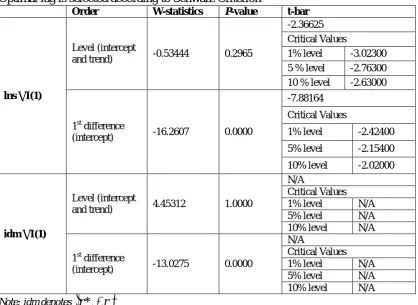
_t_₁are proven to be I(1) in both periods as shown in Table 1 and Table 2. Bothlns_i_,_tand



r*_i r



_t_₁need to be 1st differenced. Therefore, the UIP Fixed Effect Model should be transformed into the following equation,

1

Galati, Health and McGuire (2007) suggested that from 2002 to 2005, British pound is one of the popular target currencies, while Japanese Yen is a popular fund currency, i.e. people tended to short Yen and long Pound.

(5)

42

lns_i_,_t _i 



r*_i r



_t_₁e_i_,_t _i 





r*_i r



_t_₁



r*_i r



_t_₂



e_i_,_t lns_i_,_t _i 



r*_i r



_t_₁



r*_i r



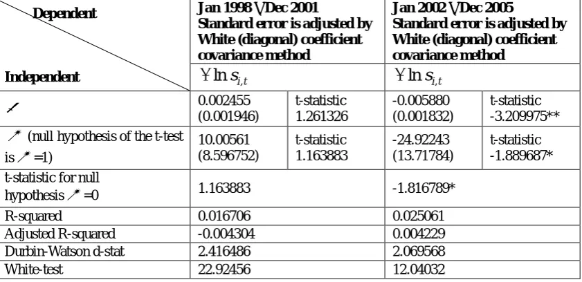
_t_₂ e_i_,_t

After rearranging, we see that the still has the original meaning2. Table 3 shows that the Durbin Watson d-statistics and the result of White test, the model in the former period suffered from serial correlation and heteroscedasticity, while in the latter period the model suffered from heteroscedasticity, so White (diagonal) coefficient covariance method is used to adjust the S.E. in order to give consistent results. Table 3 shows that we cannot reject UIP existed during the pre carry trade period from 1998 to 2001. The mean of



_iin the FEM is not significantly different from zero since the t-statistic is 1.26 and does not exceed the critical value of 5% significant level.  is not significantly different from 1, and the t-statistic with the null hypothesis =1 is 1.16, lower than the critical value of 5% significant level.

However, the carry trade period between 2002 and 2005 was completely different as shown in Table 3. UIP collapsed. The mean of



_iis significantly lower than zero by having a high t-statistic -3.21. The reason may be that holding currencies other than USD is risky, so even if there was no interest difference, USD tends to depreciate in this period. The striking point, however, is that is significantly lower than 1 at 10% significant level in this period, though the t-statistic with the null hypothesis =1 is -1.89, cannot exceed the 5% significant level critical value. Moreover,  also significantly lower than 0 at 10% significant level in this period, the t-statistic with the null hypothesis =0 is -1.82. Therefore, higher interest rate currencies tend to appreciate in the carry trade period.

Diagrammatically, Figure 1 shows the scatter graph of lns_i_,_t and (r*i r)t₁

between 1998 and 2001. There is a positive relationship suggested by UIP, though whether UIP held perfectly is not clear. Figure 2 shows the scatter graph of lns_i_,_t and (r*_i r)_t_₁ between 2002 and 2005 and they had a negative

relationship, implying that high interest rate currencies will appreciate in the future.

Now we discovered that UIP did not hold in the carry trade period. We go one step further to study the pattern of the UIP failure between 2002 and 2005 by using VAR, since both lns and (r*i – r) are I(1). And they are not co-integrated as Table 4 shows

that the residual of the liner combination of these two series has a unit root in both periods. So we apply the following fixed effect VAR forlnsand(r*_i r),3

t i k t i k t i k t i k t i i t

i s s r r r r u

s_, ₀ ₁ ln _, ₁ ... ln _, ₁ ( * ) ₁ ... ( * ) ₁_,

ln              

   _  _  _  _ t i k t i k t i k t i k t i i t

i r r r r r s s u

r* ) ₀ ₁ ( * ) ₁ ... ( * ) ₁ ln _, ₁ ... ln _, ₂_,

(               

   _  _  _  _

The optimal lag k is selected by AIC (Akaike Information Criteria) and the maximum

2_{This means that the} _{still shows the relationship between}





1 *i r _t_

r andlns_i_,_t.

3

Though the VARs is forlnsand(r*_i r), it still can show the +ve or –ve relation

(6)

43

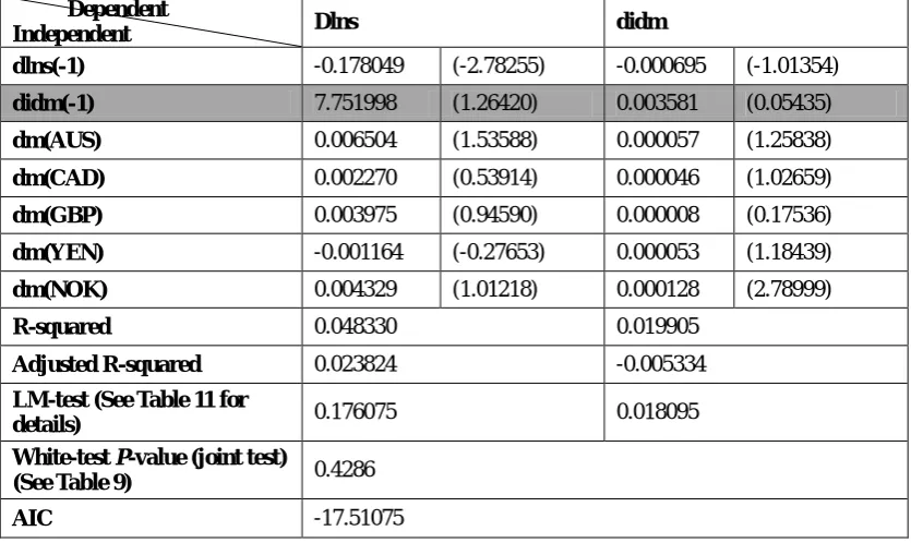
lag is 8. u₁_i_,_t and u₂_i_,_tare error terms. Table 5 shows the VAR results of the period

between 1998 and 2001, the optimal lag is 1 month. Therefore, interest rate differential, and exchange rate, did not have a long impact on each other; the market reached its equilibrium within a month. Table 6 shows the results of Granger Causality test that high P-values implied that we cannot reject interest rate differential and exchange rate did not have any causal relationship. Note that the inability of rejecting the notion that the two variables did not have any causal relationship does not mean that we can reject that they had causal relationship. Therefore, this result still does not contradict with the result of UIP FEM above.

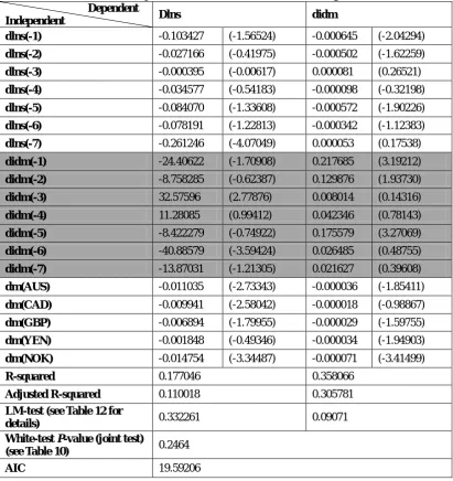
The VAR results of the carry trade period from 2002 to 2005 are very meaningful and have deep implications. Table 7 shows the result of the VAR. The optimal lag number is 7 according to AIC, implying that the market during this period took a longer time to reach the equilibrium. Table 8 reports the result of the Granger Causality test. The P-value of the Granger Causality from (r*_i r)tolns is 0.0000, while the P-value of the Granger Causality fromlns to (r*_i r)is 0.1450 and is not significant at 5% level. Therefore, between 2002 and 2005

) * (r _i r

 Granger causedlns but not the opposite. Note that LM autocorrelation test and White Heteroskedasticity test are also performed for the VARs. They do not suffer from these problems (see Table 5 and 7).

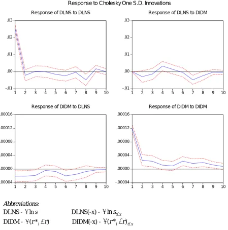
4. Analysis of the Impulse Response in the Carry Trade Period

Figure 3 shows the VAR impulse response function in terms of standard deviation of the period between 2002 and 2005. The first striking result is the response of

s

ln

 to (r*i r)was negative at the beginning, but becomes positive after 3 months. This suggests that higher interest rate currencies tend to appreciate first and then depreciate. The second important finding is the response of (r*_i r)to itself remained positive for more than ten months. This means an increase in interest rate will lead to increases in interest rate in the later periods.

A reasonable explanation for the fact that higher interest rate currencies tends to appreciate first and then depreciate is the self-fulfilling behaviour of the carry traders. Carry traders in this period discovered that higher interest rates would persist for a long period (shown by the impulse response of (r*_i r)to itself). Moreover, carry traders knew that other investors would also engage in carry trade. Hence, they built up a consensus that the demand for high interest rate currencies would remain large for a period, and the currencies would appreciate. Thus they were more willing to short low interest rate currencies and long high interest rate currencies. This behaviour caused high interest rate currencies appreciated eventually, even though there was no fundamental reason for the currency price to go up. As a result, UIP cannot hold. Nevertheless, after the appreciation, investors made a profit and tried to unwind the carry trade by selling the high interest rate currency. This explains why the high interest rate currency would appreciate first but depreciates after two or three months.

(7)

44

Reader may ask why carry traders did not act in this way in the pre carry trade period from 1998 to 2002. The reason may be because at that time carry traders still did not built up a consensus. If an investor believed that other investors would not engage in carry trade, the high interest rate currency would not appreciate or even depreciate. So, there is no point for the investor to do carry trade at the beginning. However, the fact shows that the consensus eventually was built up. Therefore, it must be that some investors started carry trade, as vanguards, and made other investors believed that carry trade was the norm. Nevertheless, this paper still did not find out the reason why those vanguards were willing to start carry trade. A noteworthy point is that even though the investors built up a consensus, and realized the carry trade profit by themselves, it is different from a coordinated game or focal point suggested by Schelling (1960). This is because the carry traders still faced a zero sum game. They sooner or later had to unwind the carry trade, and whether they could earn a profit finally, still depends on the timing of clearing the carry trade position.

Actually, higher interest rate leads to appreciation does not totally contradict to the UIP. For example, at the beginning the interest rate of the home currency and foreign currency are the same, but later the home currency interest rate increases by 3%. Assume the expected exchange rate is fixed, so home currency‟s return is higher. Therefore, investors will buy home currency until it appreciates by 3% in order to make the return of the two currencies equal. The key question is how fast this 3% appreciation happens. If it happens very slowly, it would lead to the UIP seemingly failed.

5. Conclusion and Implications

This study reveals that the behaviours and consensuses of the international financial market will change from time to time. Different behaviours and consensuses will lead to different relationship between exchange rate and other factors such as interest rate. As a result, using one or two rigid theories to generalize the operation of the ever changing market may not be effective. In addition, probably it is more appropriate to narrow down the range of time when doing empirical researches. Moreover, variables representing risk may be added for reflecting the risk premium of currencies.

References

Brennermeier Markus K., Negel Stefan and Lasse H. Pedersen (2009). “Carry Trades and Currency Crashes,” NBER Working Paper No. 14473.

Flood Robert P. and Rose Andrew K (1994). “Fixes: of the Forward Discount Puzzle.” NBER Working Paper No. 4928.

Flood Robert P. and Rose Andrew K (2001). “Uncovered Interest Parity in Crisis: The Interest Rate Defense in the 1990s.” IMF Working Paper no. 01/207.

Froot Kenneth A and Thaler Richard H (1990). “Anomalies Foreign Exchange.” The Journal of Economic Perspectives, 4, no. 3: 179-192.

Galati Gabriele, Heath Alexandra and McGuire Patrick (2007). “Evidence of carry trade activity,” Bank of International Settlement Quarterly Rewiew, September 2007, 27-41.

Plantin Guillaume and Shin Hyun Song (2008). “Carry Trades and Speculative Dynamics.” Working Paper, Princeton University.

(8)

45

McCallum Bennett T. (1992). “A Reconsideration of the Uncovered Interest Parity Relationship,” NBER Working Paper No. 4113.

Schelling Thomas C. (1980). The strategy of conflict. Cambridge: Harvard University Press.

Appendix I:

(Test result details such as White test and LM test are available subject to request)

Table 1: Im, Pesaran and Shin Panel Unit Root Test, Jan 1998 – Dec 2001 Optimal lag is selected according to Schwarz Criterion

Order W-statistics P-value t-bar

lns – I(1)

Level (intercept

and trend) -0.53444 0.2965

-2.36625

Critical Values

1% level -3.02300 5 % level -2.76300

10 % level -2.63000

1st difference

(intercept) -16.2607 0.0000

-7.88164

Critical Values

1% level -2.42400

5% level -2.15400

10% level -2.02000

idm – I(1)

Level (intercept

and trend) 4.45312 1.0000

N/A

Critical Values 1% level N/A 5% level N/A 10% level N/A

1st difference

(intercept) -13.0275 0.0000

N/A

Critical Values 1% level N/A 5% level N/A 10% level N/A Note: idm denotes





t i r

r* 

(9)

46

Table 2: Im, Pesaran and Shin Panel Unit Root Test, Jan 2002 – Dec 2005 Optimal lag is selected according to Schwarz Criterion

Order W-statistics P-value t-bar lns – I(1) Level (intercept

and trend)

1.70935 0.9563 -1.56373

Critical Values

1% level -3.02300

5 % level -2.76300

10 % level -2.63000

1st difference (intercept)

-13.2679 0.0000 -6.71176

Critical Values

1% level -2.42400

5% level -2.15400

10% level -2.02000

idm – I(1) Level (intercept and trend)

5.36188 1.0000 N/A

Critical Values 1% level N/A 5% level N/A 10% level N/A 1st difference

(intercept)

-5.46560 0.0000 N/A

Critical Values 1% level N/A 5% level N/A 10% level N/A Note: idm denotes





t i r

r* 

Table 3: Uncovered Interest Parity Fixed Effect Model – standard error in parenthesis

Dependent

Independent

Jan 1998 – Dec 2001

Standard error is adjusted by White (diagonal) coefficient covariance method

Jan 2002 – Dec 2005

Standard error is adjusted by White (diagonal) coefficient covariance method

t i s_, ln

 lns_i_,_t

 0.002455

(0.001946)

t-statistic 1.261326

-0.005880 (0.001832)

t-statistic -3.209975**

 (null hypothesis of the t-test is =1)

10.00561 (8.596752)

t-statistic 1.163883

-24.92243 (13.71784)

t-statistic -1.889687*

t-statistic for null

hypothesis =0 1.163883 -1.816789*

R-squared 0.016706 0.025061

Adjusted R-squared -0.004304 0.004229 Durbin-Watson d-stat 2.416486 2.069568

White-test 22.92456 12.04032

(10)

47

Table 4: Augment Engle-Granger Two Step Co-integration Test (none) between lnst

and idmt-1 (Use IPS penal unit root test for the residual of the linear combination of

lnst and idmt-1) Optimal lag is selected according to Schwarz Criterion

Period W-statistics P-value t-bar

Jan 1998 – Dec 2001 (rejected)

(intercept and

trend) 0.12559 0.5500

-2.12981 Critical Values

1% level -3.02400 5 % level -2.76400 10 % level -2.63000

Jan 2002 – Dec 2005 (rejected)

1st difference

(intercept) 2.419465 0.9922

-1.30797 Critical Values

1% level -3.02400 5% level -2.76400

10% level -2.63000

Table 5: Fixed Effect VAR Jan 1998 – Dec 2001, t-statistics in parenthesis Dependent

Independent Dlns didm

dlns(-1) -0.178049 (-2.78255) -0.000695 (-1.01354)

didm(-1) 7.751998 (1.26420) 0.003581 (0.05435)

dm(AUS) 0.006504 (1.53588) 0.000057 (1.25838)

dm(CAD) 0.002270 (0.53914) 0.000046 (1.02659)

dm(GBP) 0.003975 (0.94590) 0.000008 (0.17536)

dm(YEN) -0.001164 (-0.27653) 0.000053 (1.18439)

dm(NOK) 0.004329 (1.01218) 0.000128 (2.78999)

R-squared 0.048330 0.019905

Adjusted R-squared 0.023824 -0.005334

LM-test (See Table 11 for

details) 0.176075 0.018095

White-test P-value (joint test)

(See Table 9) 0.4286

AIC -17.51075

(11)

48

Table 6: Granger Causality Jan 1998 – Dec 2001 F-statistics and P-value in parenthesis

Dependent

Excluded Dlns didm

Dlns 1.027272 (0.3180)

Didm 1.598199 (0.2062)

Abbreviations:

dlns - lns dlns(-x) - lns_t_x

didm - (r*_i r) didm(-x) - (r*_i r)_t_x dm(AUS) – dummy variable for Australian Dollar. dm(CAD) – dummy variable for Canadian Dollar dm(GBP) – dummy variable for British Pound dm(YEN) – dummy variable for Japanese Yen dm(NOK) – dummy variable for Norwegian Krone

These abbreviations are also available in the following Tables.

Table 7: Fixed Effect VAR Jan 2002 – Dec 2005, t-statistics in parenthesis Dependent

Independent Dlns didm

dlns(-1) -0.103427 (-1.56524) -0.000645 (-2.04294)

dlns(-2) -0.027166 (-0.41975) -0.000502 (-1.62259)

dlns(-3) -0.000395 (-0.00617) 0.000081 (0.26521)

dlns(-4) -0.034577 (-0.54183) -0.000098 (-0.32198)

dlns(-5) -0.084070 (-1.33608) -0.000572 (-1.90226)

dlns(-6) -0.078191 (-1.22813) -0.000342 (-1.12383)

dlns(-7) -0.261246 (-4.07049) 0.000053 (0.17538)

didm(-1) -24.40622 (-1.70908) 0.217685 (3.19212)

didm(-2) -8.758285 (-0.62387) 0.129876 (1.93730)

didm(-3) 32.57596 (2.77876) 0.008014 (0.14316)

didm(-4) 11.28085 (0.99412) 0.042346 (0.78143)

didm(-5) -8.422279 (-0.74922) 0.175579 (3.27069)

didm(-6) -40.88579 (-3.59424) 0.026485 (0.48755)

didm(-7) -13.87031 (-1.21305) 0.021627 (0.39608)

dm(AUS) -0.011035 (-2.73343) -0.000036 (-1.85411)

dm(CAD) -0.009941 (-2.58042) -0.000018 (-0.98867)

dm(GBP) -0.006894 (-1.79955) -0.000029 (-1.59755)

dm(YEN) -0.001848 (-0.49346) -0.000034 (-1.94903)

dm(NOK) -0.014754 (-3.34487) -0.000071 (-3.41499)

R-squared 0.177046 0.358066

Adjusted R-squared 0.110018 0.305781

LM-test (see Table 12 for

details) 0.332261 0.09071

White-test P-value (joint test)

(see Table 10) 0.2464

AIC 19.59206

(12)

49

Table 8: Granger Causality Jan 2002 – Dec 2005 F-statistics and P-value in parenthesis

Dependent

Excluded Dlns didm

Dlns 10.85663 (0.1450)

Didm 32.29167 (0.0000)

Example 1: Case A – YEN GBP carry trade profit from 1998 to 2001

Time

Yen to GBP exchange rate

YEN inter-bank one month interest rate divided by 12

GBP inter-bank one month interest rate divided by 12

YEN one month interest return minus GBP one month interest return

The cumulative wealth using carry trade strategy

The cumulative wealth of investing in YEN only

1/1/1998 215.5332 0.000834 0.006198 -0.00536 100 100

1/2/1998 207.4414 0.000697 0.006172 -0.00547 96.84222 100.0834

1/3/1998 206.6678 0.00103 0.006185 -0.00516 97.07652 100.1532

1/4/1998 223.4331 0.00059 0.006185 -0.00559 105.6007 100.2563

1/5/1998 222.3426 0.00051 0.006068 -0.00556 105.7352 100.3154

1/6/1998 229.1762 0.000465 0.006146 -0.00568 109.6462 100.3665

1/7/1998 228.9889 0.000608 0.006263 -0.00566 110.2299 100.4132

1/8/1998 236.9123 0.000558 0.00625 -0.00569 114.7583 100.4742

1/9/1998 228.5523 0.000685 0.00625 -0.00556 111.4007 100.5303

1/10/1998 231.5368 0.000458 0.00612 -0.00566 113.5608 100.5992

1/11/1998 191.2646 0.000439 0.006042 -0.0056 94.38274 100.6452

1/12/1998 201.9848 0.000614 0.005729 -0.00512 100.275 100.6895

1/1/1999 188.2675 0.000481 0.005156 -0.00467 94.00057 100.7513

1/2/1999 188.8542 0.000414 0.004896 -0.00448 94.77972 100.7998

1/3/1999 192.7767 0.000376 0.00457 -0.00419 97.22194 100.8415

1/4/1999 193.251 0.000153 0.00431 -0.00416 97.90659 100.8795

1/5/1999 193.4975 0.000118 0.004349 -0.00423 98.45396 100.8949

1/6/1999 194.4391 8.53E-05 0.004362 -0.00428 99.3633 100.9068

1/7/1999 190.118 8.93E-05 0.004167 -0.00408 97.57893 100.9154

1/8/1999 185.0049 8.21E-05 0.004323 -0.00424 95.35021 100.9244

1/9/1999 175.3249 8.51E-05 0.004141 -0.00406 90.75185 100.9327

1/10/1999 173.9987 7.86E-05 0.004479 -0.0044 90.43831 100.9413

1/11/1999 171.0319 7.56E-05 0.004479 -0.0044 89.29445 100.9492

1/12/1999 164.4573 0.000726 0.004818 -0.00409 86.24648 100.9568

1/1/2000 166.3392 0.000132 0.004323 -0.00419 87.65371 101.0301

1/2/2000 174.1201 7.92E-05 0.005 -0.00492 92.15055 101.0434

1/3/2000 170.046 0.000105 0.005 -0.0049 90.44436 101.0514

1/4/2000 167.6151 9.58E-05 0.004935 -0.00484 89.59716 101.062

(13)

50 Time

1/6/2000 162.0798 7.44E-05 0.004948 -0.00487 87.50572 101.0797

1/7/2000 159.8698 0.000136 0.004948 -0.00481 86.73964 101.0872

1/8/2000 162.9812 0.000108 0.004974 -0.00487 88.8653 101.101

1/9/2000 155.1179 0.000342 0.004974 -0.00463 84.99853 101.1119

1/10/2000 159.5979 0.000306 0.005 -0.00469 87.88839 101.1465

1/11/2000 157.0786 0.000286 0.004896 -0.00461 86.93353 101.1774

1/12/2000 160.3836 0.000579 0.004896 -0.00432 89.19725 101.2064

1/1/2001 171.1026 0.000453 0.004818 -0.00436 95.62451 101.2649

1/2/2001 170.5752 0.000355 0.004844 -0.00449 95.78901 101.3108

1/3/2001 170.7697 0.00027 0.004714 -0.00444 96.36274 101.3467

1/4/2001 179.6738 9.49E-05 0.004635 -0.00454 101.8651 101.374

1/5/2001 175.1722 6.09E-05 0.004427 -0.00437 99.77327 101.3837

1/6/2001 169.0574 5.19E-05 0.004271 -0.00422 96.71676 101.3898

1/7/2001 175.8821 5.71E-05 0.004271 -0.00421 101.0509 101.3951

1/8/2001 178.6032 5.45E-05 0.004323 -0.00427 103.0525 101.4009

1/9/2001 172.7312 5.9E-05 0.00401 -0.00395 100.0953 101.4064

1/10/2001 176.7672 5.06E-05 0.003854 -0.0038 102.8449 101.4124

1/11/2001 178.4377 5.06E-05 0.003438 -0.00339 104.2169 101.4175

1/12/2001 176.698 7.63E-05 0.003292 -0.00322 103.5556 101.4227

The case calculates the cumulative YEN return of a carry trader and a YEN investor, both of them have 100 YEN at the beginning. The YEN investor invested in YEN only, so each month he received the YEN interest return only. For example, the wealth of the YEN investor‟s wealth in 1/2/1998 was 100YEN*(1+0.000834) = 100.0834YEN. The cumulative wealth of the YEN investor is shown on the last column of the table above.

The carry trader invested in a higher interest rate currency in each month. Also assume he could only choose YEN and GBP. Therefore, at the beginning of each month, he chose the higher interest rate currency from YEN or GBP. If GBP offered a high rate, he would invest in GBP. At the end of the month he would convert the GBP back into YEN. And see whether GBP or YEN offered a higher rate in the next month, then invest in a higher interest rate currency again.

From 1998 to 2001 when the interest rate of GBP was always higher than YEN the carry trader at the first month converted YEN to GBP, and invested in GBP deposit. A t the end of the month, he converted the GBP back to YEN. At the beginning of the second month, he converted YEN to GBP and invested in GBP again for a month. He was repeating this action until 1/12/2001. The cumulative wealth is report at the

(14)

51

second last column of the table. For example, the wealth of the carry trader in 1/2/1998 was (100YEN/215.5332)*(1+0.006198)*207.4414=96.84222.

Case B – YEN GBP carry trade profit from 2002 to 2005

Time

1/1/2002 190.6769 5.77E-05 0.003412 -0.00335 100 100

1/2/2002 188.3657 5.14E-05 0.003307 -0.00326 99.12492 100.0058

1/3/2002 189.2578 0.000124 0.003333 -0.00321 99.9238 100.0109

1/4/2002 192.2069 8.13E-05 0.003307 -0.00323 101.8191 100.0233

1/5/2002 186.6813 5.97E-05 0.003229 -0.00317 99.21907 100.0314

1/6/2002 181.0158 5.14E-05 0.003333 -0.00328 96.51859 100.0374

1/7/2002 183.6553 4.79E-05 0.003281 -0.00323 98.25241 100.0425

1/8/2002 186.1202 4.44E-05 0.003229 -0.00318 99.89781 100.0473

1/9/2002 182.928 6.04E-05 0.003307 -0.00325 98.50145 100.0518

1/10/2002 191.7917 4.72E-05 0.003229 -0.00318 103.6159 100.0578

1/11/2002 191.338 4.72E-05 0.003229 -0.00318 103.7046 100.0625

1/12/2002 194.0869 6.53E-05 0.003307 -0.00324 105.5342 100.0672

1/1/2003 191.1717 5.07E-05 0.003333 -0.00328 104.2928 100.0738

1/2/2003 197.65 4.93E-05 0.003333 -0.00328 108.1864 100.0789

1/3/2003 185.7549 0.000075 0.00306 -0.00298 102.0144 100.0838

1/4/2003 186.2948 5.14E-05 0.003021 -0.00297 102.624 100.0913

1/5/2003 191.0277 0.00005 0.002917 -0.00287 105.5491 100.0964

1/6/2003 194.1398 0.00005 0.003047 -0.003 107.5815 100.1014

1/7/2003 198.3962 0.00005 0.003021 -0.00297 110.2751 100.1064

1/8/2003 193.6825 0.00005 0.002813 -0.00276 107.9803 100.1115

1/9/2003 183.315 6.88E-05 0.002995 -0.00293 102.4877 100.1165

1/10/2003 184.5769 0.00005 0.003021 -0.00297 103.5023 100.1233

1/11/2003 185.9742 0.00005 0.003073 -0.00302 104.6008 100.1283

1/12/2003 188.0887 5.83E-05 0.003151 -0.00309 106.1152 100.1334

1/1/2004 191.4122 0.00005 0.003177 -0.00313 108.3306 100.1392

1/2/2004 192.4276 0.00005 0.003281 -0.00323 109.2512 100.1442

1/3/2004 203.7678 5.97E-05 0.003412 -0.00335 116.0693 100.1492

1/4/2004 192.6026 0.00005 0.003385 -0.00334 110.0837 100.1552

1/5/2004 195.2959 0.00005 0.003516 -0.00347 112.0009 100.1602

1/6/2004 203.2101 0.00005 0.003672 -0.00362 116.9494 100.1652

(15)

52 Time

1/8/2004 202.2536 0.00005 0.00388 -0.00383 117.2705 100.1752

1/9/2004 196.2249 5.83E-05 0.003984 -0.00393 114.2164 100.1802

1/10/2004 198.7592 0.00005 0.003984 -0.00393 116.1526 100.1861

1/11/2004 195.2054 0.00005 0.003984 -0.00393 114.5302 100.1911

1/12/2004 198.5786 5.69E-05 0.003984 -0.00393 116.9736 100.1961

1/1/2005 195.9508 5.07E-05 0.00401 -0.00396 115.8856 100.2018

1/2/2005 195.2448 0.00005 0.003984 -0.00393 115.9311 100.2069

1/3/2005 200.4513 6.6E-05 0.00401 -0.00394 119.4969 100.2119

1/4/2005 202.4177 5.14E-05 0.00401 -0.00396 121.153 100.2185

1/5/2005 199.2515 0.00005 0.004023 -0.00397 119.7362 100.2237

1/6/2005 196.7301 0.00005 0.003984 -0.00393 118.6967 100.2287

1/7/2005 197.5959 0.00005 0.003932 -0.00388 119.6941 100.2337

1/8/2005 198.5598 4.93E-05 0.003802 -0.00375 120.751 100.2387

1/9/2005 201.3843 5.9E-05 0.003776 -0.00372 122.9343 100.2436

1/10/2005 200.3071 0.00005 0.003776 -0.00373 122.7384 100.2495

1/11/2005 206.1937 0.00005 0.003789 -0.00374 126.8225 100.2546

1/12/2005 208.6855 5.69E-05 0.003776 -0.00372 128.8415 100.2596

The logic is the same as Case A.

Reminder 1 – details of the one month interest rate

The 1-month interest rate of U.S. dollar is the 1-month interest rate in the certificate deposit secondary market of the U.S. The 1 month interest rate of Australian dollar is 1-month inter-bank interest rate in Australia. The 1-month interest rate of Canadian dollar is the 1-month interest rate of Treasury Bills of Canada. The 1-month interest rate of British pound is the 1-month inter-bank interest rate of the United Kingdom. The 1-month interest rate of Japanese Yen is the 1-month inter-bank interest rate in Japan. The 1-month interest rate of Norwegian Krone is the 1-month inter-bank interest rate in Norway. Though some of them are slightly different, all of them represent the risk-free and highly liquid interest rate. Since they are annualized interest rates, in the regression of this paper all of them are divided by 12 in order to reflect the monthly interest returns of each currency.

(16)

53

Figure 1: Scatter Diagram of lns_i_,_tand(r*_i r)_t_₁, Jan 1998 – Dec 2001

-.08 -.04 .00 .04 .08 .12

-.0010 -.0005 .0000 .0005 .0010

DIDM(t-1)

DL

N

S

(t)

AUS

-.04 -.02 .00 .02 .04

-.0010 -.0005 .0000 .0005 .0010

DIDM(t-1)

DL

N

S

(t)

CAD

-.04 -.02 .00 .02 .04

-.0010 -.0005 .0000 .0005 .0010

DIDM(t-1)

D

L

N

S

(t)

GBP

-.20 -.15 -.10 -.05 .00 .05 .10

-.0005 .0000 .0005 .0010

DIDM(t-1)

D

L

N

S

(t)

YEN

-.06 -.04 -.02 .00 .02 .04 .06

-.001 .000 .001 .002 .003

DIDM(t-1)

D

L

NS

(t

)

NOK

(17)

54

Figure 2: Scatter Diagram of lns_i_,_tand(r*_i r)_t_₁, Jan 2002 – Dec 2005

-.08 -.04 .00 .04 .08

-.0004 -.0002 .0000 .0002 .0004

DIDM(t-1)

DL

N

S

(t)

AUS

-.04 -.02 .00 .02 .04 .06

-.0004 -.0002 .0000 .0002 .0004

DIDM(t-1)

DL

N

S

(t)

CAD

-.08 -.06 -.04 -.02 .00 .02 .04 .06

-.0004 -.0002 .0000 .0002 .0004

DIDM(t-1)

D

L

N

S

(t)

GBP

-.06 -.04 -.02 .00 .02 .04 .06 .08

-.0004 -.0002 .0000 .0002 .0004

DIDM(t-1)

D

L

N

S

(t)

YEN

-.08 -.04 .00 .04 .08

-.0008 -.0004 .0000 .0004

DIDM(t-1)

D

L

NS

(t

)

NOK

(18)

55 -.01

.00 .01 .02 .03

1 2 3 4 5 6 7 8 9 10 Response of DLNS to DLNS

-.01 .00 .01 .02 .03

1 2 3 4 5 6 7 8 9 10 Response of DLNS to DIDM

-.00004 .00000 .00004 .00008 .00012 .00016

1 2 3 4 5 6 7 8 9 10 Response of DIDM to DLNS

-.00004 .00000 .00004 .00008 .00012 .00016

1 2 3 4 5 6 7 8 9 10 Response of DIDM to DIDM

Response to Cholesky One S.D. Innovations

Figure 3: Impulse response in terms of 1 standard deviation, 2002-2005

Abbreviations:

DLNS - lns DLNS(-x) - lns_t__x

DIDM - (r*_i r) DIDM(-x) - (r*_i r)_t__x

(19)

56