Contents
1 High-Dimensional Space 2
1.1 Properties of High-Dimensional Space . . . 4
1.2 The High-Dimensional Sphere . . . 5
1.2.1 The Sphere and the Cube in Higher Dimensions . . . 5
1.2.2 Volume and Surface Area of the Unit Sphere . . . 6
1.2.3 The Volume is Near the Equator . . . 9
1.2.4 The Volume is in a Narrow Annulus . . . 11
1.2.5 The Surface Area is Near the Equator . . . 11
1.3 The High-Dimensional Cube and Chernoff Bounds . . . 13
1.4 Volumes of Other Solids . . . 18
1.5 Generating Points Uniformly at Random on the surface of a Sphere . . . . 19
1.6 Gaussians in High Dimension . . . 20
1.7 Random Projection and the Johnson-Lindenstrauss Theorem . . . 26
1.8 Bibliographic Notes . . . 29
1
High-Dimensional Space
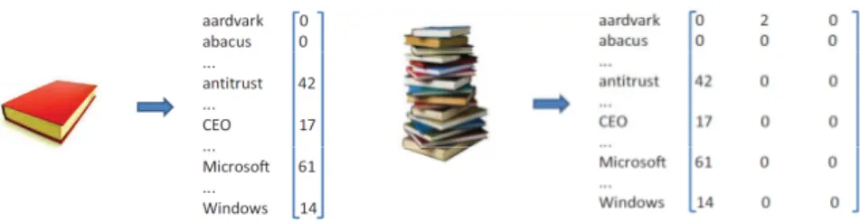
Consider representing a document by a vector each component of which corresponds to the number of occurrences of a particular word in the document. The English language has on the order of 25,000 words. Thus, such a document is represented by a 25,000-dimensional vector. The representation of a document is called theword vector model [?]. A collection ofndocuments may be represented by a collection of 25,000-dimensional vec-tors, one vector per document. The vectors may be arranged as columns of a 25,000×n matrix.
Another example of high-dimensional data arises in customer-product data. If there are 1,000 products for sale and a large number of customers, recording the number of times each customer buys each product results in a collection of 1,000-dimensional vec-tors.
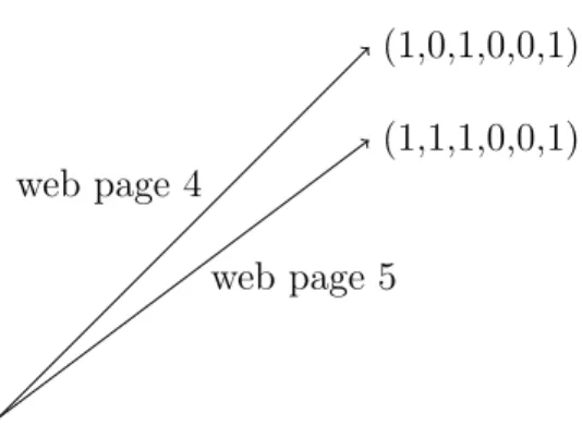
There are many other examples where each record of a data set is represented by a high-dimensional vector. Consider a collection of n web pages that are linked. A link is a pointer from one web page to another. Each web page can be represented by a 0-1 vector with n components where the jth component of the vector representing the ith
web page has value 1, if and only if there is a link from theithweb page to thejthweb page. In the vector space representation of data, properties of vectors such as dot products, distance between vectors, and orthogonality often have natural interpretations. For ex-ample, the squared distance between two 0-1 vectors representing links on web pages is the number of web pages to which only one of them is linked. In Figure 1.2, pages 4 and 5 both have links to pages 1, 3, and 6 but only page 5 has a link to page 2. Thus, the squared distance between the two vectors is one.
When a new web page is created a natural question is which are the closest pages to it, that is the pages that contain a similar set of links. This question translates to the geometric question of finding nearest neighbors. The nearest neighbor query needs to be answered quickly. Later in this chapter we will see a geometric theorem, called the Random Projection Theorem, that helps with this. If each web page is a d-dimensional vector, then instead of spending timedto read the vector in its entirety, once the random projection to ak-dimensional space is done, one needs only readk entries per vector.
Dot products also play a useful role. In our first example, two documents containing many of the same words are considered similar. One way to measure co-occurrence of words in two documents is to take the dot product of the vectors representing the two documents. If the most frequent words in the two documents co-occur with similar fre-quencies, the dot product of the vectors will be close to the maximum, namely the product of the lengths of the vectors. If there is no co-occurrence, then the dot product will be close to zero. Here the objective of the vector representation is information retrieval.
Figure 1.1: A document and its term-document vector along with a collection of docu-ments represented by their term-document vectors.
After preprocessing the document vectors, we are presented with queries and we want to find for each query the most relevant documents. A query is also represented by a vector which has one component per word; the component measures how important the word is to the query. As a simple example, to find documents about cars that are not race cars, a query vector will have a large positive component for the word car and also for the words engine and perhaps door and a negative component for the words race, betting, etc. Here dot products represent relevance.
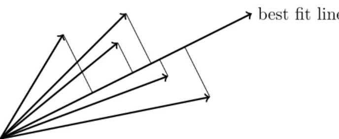
An important task for search algorithms is to rank a collection of web pages in order of relevance to the collection. An intrinsic notion of relevance is that a document in a collection is relevant if it is similar to the other documents in the collection. To formalize this, one can define an ideal direction for a collection of vectors as the line of best-fit, or the line of least-squares fit, i.e., the line for which the sum of squared perpendicular distances of the vectors to it is minimized. Then, one can rank the vectors according to their dot product similarity with this unit vector. We will see in Chapter ?? that this is a well-studied notion in linear algebra and that there are efficient algorithms to find the line of best fit. Thus, this ranking can be efficiently done. While the definition of rank seems ad-hoc, it yields excellent results in practice and has become a workhorse for modern search, information retrieval, and other applications.
Notice that in these examples, there was no intrinsic geometry or vectors, just a collection of documents, web pages or customers. Geometry was added and is extremely useful. Our aim in this book is to present the reader with the mathematical foundations to deal with high-dimensional data. There are two important parts of this foundation. The first is high-dimensional geometry along with vectors, matrices, and linear algebra. The second more modern aspect is the combination with probability. When there is a stochastic model of the high-dimensional data, we turn to the study of random points. Again, there are domain-specific detailed stochastic models, but keeping with our objective of introducing the foundations, the book presents the reader with the mathematical results needed to tackle the simplest stochastic models, often assuming independence and uniform or Gaussian distributions.
web page 4
(1,0,1,0,0,1)
web page 5
(1,1,1,0,0,1)
Figure 1.2: Two web pages as vectors. The squared distance between the two vectors is the number of web pages linked to by just one of the two web pages.
1.1
Properties of High-Dimensional Space
Our intuition about space was formed in two and three dimensions and is often mis-leading in high dimensions. Consider placing 100 points uniformly at random in a unit square. Each coordinate is generated independently and uniformly at random from the interval [0, 1]. Select a point and measure the distance to all other points and observe the distribution of distances. Then increase the dimension and generate the points uni-formly at random in a 100-dimensional unit cube. The distribution of distances becomes concentrated about an average distance. The reason is easy to see. Let x and y be two such points ind-dimensions. The distance betweenx and y is
|x−y|=
v u u t
d X
i=1
(xi−yi)2.
Since Pdi=1(xi−yi)2 is the summation of a number of independent random variables of
bounded variance, by the law of large numbers the distribution of|x−y|2 is concentrated about its expected value. Contrast this with the situation where the dimension is two or three and the distribution of distances is spread out.
For another example, consider the difference between picking a point uniformly at random from the unit-radius circle and from a unit radius sphere in d-dimensions. In d-dimensions the distance from the point to the center of the sphere is very likely to be between 1− c
d and 1, where c is a constant independent of d. Furthermore, the first
coordinate, x1, of such a point is likely to be between −√cd and +√cd, which we express
by saying that most of the mass is near the equator. The equator perpendicular to the x1 axis is the set {x|x1 = 0}. We will prove these facts in this chapter.
best fit line
Figure 1.3: The best fit line is that line that minimizes the sum of perpendicular distances squared.
1.2
The High-Dimensional Sphere
One of the interesting facts about a unit-radius sphere in high dimensions is that as the dimension increases, the volume of the sphere goes to zero. This has important implications. Also, the volume of a high-dimensional sphere is essentially all contained in a thin slice at the equator and is simultaneously contained in a narrow annulus at the surface. There is essentially no interior volume. Similarly, the surface area is essentially all at the equator. These facts are contrary to our two or three-dimensional intuition; they will be proved by integration.
1.2.1 The Sphere and the Cube in Higher Dimensions
Consider the difference between the volume of a cube with unit-length sides and the volume of a unit-radius sphere as the dimensiond of the space increases. As the dimen-sion of the cube increases, its volume is always one and the maximum possible distance between two points grows as √d. In contrast, as the dimension of a unit-radius sphere increases, its volume goes to zero and the maximum possible distance between two points stays at two.
Note that for d=2, the unit square centered at the origin lies completely inside the unit-radius circle. The distance from the origin to a vertex of the square is
q
(1 2)
2
+(1 2)
2
=
√
2 2 ∼= 0.707
and thus the square lies inside the circle. Atd=4, the distance from the origin to a vertex of a unit cube centered at the origin is
q
(1 2)
2
+(1 2)
2
+(1 2)
2
+(1 2)
2
= 1
and thus the vertex lies on the surface of the unit 4-sphere centered at the origin. As the dimension√ d increases, the distance from the origin to a vertex of the cube increases as
d
2 , and for large d, the vertices of the cube lie far outside the unit sphere. Figure 1.5
illustrates conceptually a cube and a sphere. The vertices of the cube are at distance
√
d
1
1 2
√
2
1
1 2
1
1
1 2
q d
2
Figure 1.4: Illustration of the relationship between the sphere and the cube in 2, 4, and d-dimensions.
1
1 2
q d
2
Unit sphere Nearly all of the volume
Vertex of hypercube
Figure 1.5: Conceptual drawing of a sphere and a cube.
from the origin and for large d lie outside the unit sphere. On the other hand, the mid point of each face of the cube is only distance 1/2 from the origin and thus is inside the sphere. For large d, almost all the volume of the cube is located outside the sphere. 1.2.2 Volume and Surface Area of the Unit Sphere
For fixed dimension d, the volume of a sphere is a function of its radius and grows as rd. For fixed radius, the volume of a sphere is a function of the dimension of the space.
What is interesting is that the volume of a unit sphere goes to zero as the dimension of the sphere increases.
rdr
dΩ rd−1dΩ
dr
Figure 1.6: Infinitesimal volume ind-dimensional sphere of unit radius.
coordinates. In Cartesian coordinates the volume of a unit sphere is given by
V (d) =
x1=1
Z
x1=−1
x2=
√
1−x2 1
Z
x2=−
√
1−x2 1
· · ·
xd=√1−x2
1−···−x2d−1
Z
xd=− √
1−x2
1−···−x2d−1
dxd· · ·dx2dx1.
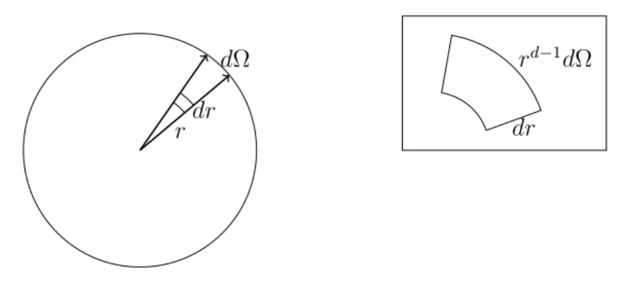
Since the limits of the integrals are complex, it is easier to integrate using polar coordi-nates. In polar coordinates, V(d) is given by
V (d) =
Z
Sd
1
Z
r=0
rd−1dΩdr.
Here, dΩ is the surface area of the infinitesimal piece of the solid angle Sd of the unit
sphere. See Figure 1.6. The convex hull of the dΩ piece and the origin form a cone. At radius r, the surface area of the top of the cone is rd−1dΩ since the surface area is d−1 dimensional and each dimension scales byr. The volume of the infinitesimal piece is base times height, and since the surface of the sphere is perpendicular to the radial direction at each point, the height isdr giving the above integral.
Since the variables Ω andr do not interact,
V (d) =
Z
Sd
dΩ
1
Z
r=0
rd−1dr = 1 d
Z
Sd
dΩ = A(d) d . The question remains, how to determine the surface areaA(d) = R
Sd
dΩ? Consider a different integral
I(d) =
∞
Z
−∞ ∞
Z
−∞
· · ·
∞
Z
−∞
e−(x21+x22+···x2d)dx
Including the exponential allows one to integrate to infinity rather than stopping at the surface of the sphere. Thus, I(d) can be computed by integrating in Cartesian coordi-nates. Integrating in polar coordinates relates I(d) to the surface area A(d). Equating the two results for I(d) givesA(d).
First, calculate I(d) by integration in Cartesian coordinates.
I(d) =
∞
Z
−∞
e−x2dx
d
= √πd=πd2
Next, calculate I(d) by integrating in polar coordinates. The volume of the differential element isrd−1dΩdr. Thus
I(d) =
Z
Sd
dΩ
∞
Z
0
e−r2rd−1dr.
The integral R Sd
dΩ is the integral over the entire solid angle and gives the surface area, A(d), of a unit sphere. Thus, I(d) = A(d)
∞
R
0
e−r2rd−1dr. Evaluating the remaining integral gives
∞
Z
0
e−r2rd−1dr = 1 2
∞
Z
0
e−ttd2 −1dt= 1
2Γ
d 2
and hence, I(d) =A(d)12Γ d2 where the gamma function Γ (x) is a generalization of the factorial function for noninteger values of x. Γ (x) = (x−1) Γ (x−1), Γ (1) = Γ (2) = 1, and Γ 12=√π. For integer x, Γ (x) = (x−1)!.
Combining I(d) = πd2 with I(d) = A(d)1 2Γ
d
2
yields
A(d) = π
d
2 1 2Γ
d
2
.
This establishes the following lemma.
Lemma 1.1 The surface area A(d) and the volume V(d) of a unit-radius sphere in d-dimensions are given by
A(d) = 2π
d
2
Γ d2 and V (d) = πd2
d
2Γ
d
2
To check the formula for the volume of a unit sphere, note that V (2) = π and V (3) = 23 π
3 2
Γ(3 2)
= 43π, which are the correct volumes for the unit spheres in two and three dimensions. To check the formula for the surface area of a unit sphere, note that A(2) = 2π and A(3) = 2π
3 2 1 2
√
π = 4π, which are the correct surface areas for the unit sphere
in two and three dimensions. Note thatπd2 is an exponential in d
2 and Γ
d
2
grows as the factorial of d2. This implies that lim
d→∞V(d) = 0, as claimed.
1.2.3 The Volume is Near the Equator
Consider a high-dimensional unit sphere and fix the North Pole on the x1 axis at
x1 = 1. Divide the sphere in half by intersecting it with the plane x1 = 0. The
in-tersection of the plane with the sphere forms a region of one lower dimension, namely
{x| |x| ≤1, x1 = 0} which we call the equator. The intersection is a sphere of dimension
d-1 and has volume V (d−1). In three dimensions this region is a circle, in four dimen-sions the region is a three-dimensional sphere, etc. In general, the intersection is a sphere of dimension d−1.
It turns out that essentially all of the mass of the upper hemisphere lies between the plane x1 = 0 and a parallel plane, x1 = ε, that is slightly higher. For what value of ε
does essentially all the mass lie between x1 = 0 and x1 =ε? The answer depends on the
dimension. For dimensiondit isO(√1
d−1). To see this, calculate the volume of the portion
of the sphere above the slice lying betweenx1 = 0 andx1 =ε. LetT ={x| |x| ≤1, x1 ≥ε}
be the portion of the sphere above the slice. To calculate the volume of T, integrate over x1 from ε to 1. The incremental volume is a disk of width dx1 whose face is a sphere of
dimension d-1 of radius p1−x2
1 (see Figure 1.7) and, therefore, the surface area of the
disk is
1−x21
d−1
2 V (d−1).
Thus,
Volume (T) =
1
Z
ε
1−x21
d−1
2 V (d−1)dx
1 =V (d−1) 1
Z
ε
1−x21
d−1
2 dx
1.
Note that V (d) denotes the volume of the d-dimensional unit sphere. For the volume of other sets such as the set T, we use the notation Volume(T) for the volume. The above integral is difficult to evaluate so we use some approximations. First, we use the inequality 1 +x ≤ ex for all real x and change the upper bound on the integral to be
infinity. Since x1 is always greater than ε over the region of integration, we can insert
x1/ε in the integral. This gives
Volume (T)≤V (d−1)
∞
Z
ε
e−d
−1
2 x
2
1dx1 ≤V(d−1) ∞
Z
ε
x1
ε e
−d−1
2 x
2 1dx1.
1 x1
dx1
p
1−x2
1 radius
(d−1)-dimensional sphere
Figure 1.7: The volume of a cross-sectional slab of a d-dimensional sphere.
Now,R x1e−
d−1 2 x
2 1 dx
1 =−d−11 e −d−21x2
1 and, hence,
Volume (T)≤ 1
ε(d−1)e −d−1
2 ε 2
V (d−1). (1.1)
Next, we lower bound the volume of the entire upper hemisphere. Clearly the volume of the upper hemisphere is at least the volume between the slabs x1 = 0 and x1 = √d1−1,
which is at least the volume of the cylinder of radius q1− 1
d−1 and height 1 √
d−1. The
volume of the cylinder is 1/√d−1 times the d−1-dimensional volume of the disk R =
{x| |x| ≤1;x1 = √d1−1}. NowR is a d−1-dimensional sphere of radius
q
1− 1
d−1 and so
its volume is
Volume(R) =V(d−1)
1− 1
d−1
(d−1)/2
. Using (1−x)a ≥1−ax
Volume(R)≥V(d−1)
1− 1
d−1 d−1
2
= 1
2V(d−1). Thus, the volume of the upper hemisphere is at least 2√1
d−1V(d−1). The fraction of
the volume above the plane x1 =ε is upper bounded by the ratio of the upper bound on
the volume of the hemisphere above the plane x1 = ε to the lower bound on the total
volume. This ratio is 2
ε√(d−1)e −d−21ε2
which leads to the following lemma.
Lemma 1.2 For anyc >0, the fraction of the volume of the hemisphere above the plane x1 = √dc−1 is less than 2ce−c
2/2
. Proof: Substitute √c
d−1 forε in the above.
For a large constantc, 2ce−c2/2
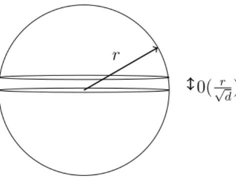
is small. The important item to remember is that most of the volume of thed-dimensional sphere of radiusr lies within distanceO(r/√d) of the
r
0(√r
d)
Figure 1.8: Most of the volume of the d-dimensional sphere of radius r is within distance O(√r
d) of the equator.
equator as shown in Figure 1.8.
For c ≥ 2, the fraction of the volume of the hemisphere above x1 = √dc−1 is less
than e−2 ≈ 0.14 and for c ≥ 4 the fraction is less than 21e−8 ≈ 3×10⁻⁴. Essentially all the mass of the sphere lies in a narrow slice at the equator. Note that we selected a unit vector in thex1 direction and defined the equator to be the intersection of the sphere with
a (d −1)-dimensional plane perpendicular to the unit vector. However, we could have selected an arbitrary point on the surface of the sphere and considered the vector from the center of the sphere to that point and defined the equator using the plane through the center perpendicular to this arbitrary vector. Essentially all the mass of the sphere lies in a narrow slice about this equator also.
1.2.4 The Volume is in a Narrow Annulus
The ratio of the volume of a sphere of radius 1−ε to the volume of a unit sphere in d-dimensions is
(1−ε)dV(d)
V(d) = (1−ε)
d
and thus goes to zero asdgoes to infinity, whenε is a fixed constant. In high dimensions, all of the volume of the sphere is concentrated in a narrow annulus at the surface.
Indeed, (1−ε)d≤e−εd, so ifε= c
d, for a large constantc, all bute
−c of the volume of
the sphere is contained in a thin annulus of widthc/d. The important item to remember is that most of the volume of the d-dimensional sphere of radiusr < 1 is contained in an annulus of widthO(1−r/d) near the boundary.
1.2.5 The Surface Area is Near the Equator
Just as a 2-dimensional circle has an area and a circumference and a 3-dimensional sphere has a volume and a surface area, ad-dimensional sphere has a volume and a surface area. The surface of the sphere is the set{x| |x|= 1}. The surface of the equator is the
1
Annulus of width 1d
Figure 1.9: Most of the volume of thed-dimensional sphere of radius r is contained in an annulus of widthO(r/d) near the boundary.
setS ={x| |x|= 1, x1 = 0} and it is the surface of a sphere of one lower dimension, i.e.,
for a 3-dimensional sphere, the circumference of a circle. Just as with volume, essentially all the surface area of a high-dimensional sphere is near the equator. To see this, calculate the surface area of the slice of the sphere betweenx1 = 0 and x1 =ε.
LetS ={x| |x|= 1, x1 ≥ε}. To calculate the surface area ofS, integrate overx1 from
εto 1. The incremental surface unit will be a band of widthdx1 whose edge is the surface
area of a d−1-dimensional sphere of radius depending on x1. The radius of the band is
p
1−x2
1 and therefore the surface area of the (d−1)-dimensional sphere is
A(d−1) 1−x21
d−2 2
whereA(d−1) is the surface area of a unit sphere of dimension d−1. Thus,
Area (S) = A(d−1)
1
Z
ε
1−x21
d−2
2 dx
1.
Again the above integral is difficult to integrate and the same approximations as in the earlier section on volume leads to the bound
Area (S)≤ 1
ε(d−2)e −d−2
2 ε 2
A(d−1). (1.2)
Next we lower bound the surface area of the entire upper hemisphere. Clearly the surface area of the upper hemisphere is greater than the surface area of the side of ad-dimensional cylinder of height √1
d−2 and radius
q
1− 1
d−2. The surface area of the cylinder is 1 √
d−2
times the circumference area of the d-dimensional cylinder of radius
q
1− 1
d−2 which is
A(d−1)(1− 1
d−2)
d−2
most
1
√
d−2(1− 1 d−2)
d−2
2 A(d−1)≥ √ 1
d−2(1− d−2
2 1
d−2)A(d−1)
≥ 1
2√d−2A(d−1) (1.3)
Comparing the upper bound on the surface area ofS, in (1.2), with the lower bound on the surface area of the hemisphere in (1.3), we see that the surface area above the band
{x| |x|= 1,0≤x1 ≤ε} is less than ε√2d−2e −d−2
2 ε 2
of the total surface area.
Lemma 1.3 For anyc >0, the fraction of the surface area above the plane x1 = √dc−2 is
less than or equal to 2ce−c
2
2 .
Proof: Substitute √c
d−2 forε in the above.
So far we have considered unit-radius spheres of dimension d. Now fix the dimension dand vary the radiusr. LetV(d, r) denote the volume and letA(d, r) denote the surface area of ad-dimensional sphere. Then,
V(d, r) =
Z r
x=0
A(d, x)dx.
Thus, it follows that the surface area is the derivative of the volume with respect to the radius. In two dimensions the volume of a circle isπr2 and the circumference is 2πr. In
three dimensions the volume of a sphere is 43πr3 and the surface area is 4πr2.
1.3
The High-Dimensional Cube and Chernoff Bounds
We can ask the same questions about the d-dimensional unit cube C = {x|0≤ xi ≤
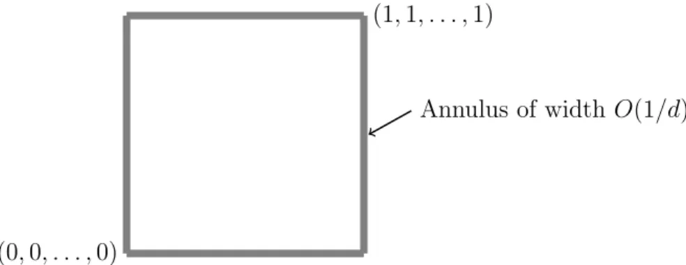
1, i= 1,2, . . . , d}as we did for spheres. First, is the volume concentrated in an annulus? The answer to this question is simple. If we shrink the cube from its center (12,12, . . . ,12) by a factor of 1−(c/d) for some constant c, the volume clearly shrinks by (1−(c/d))d≤e−c, so much of the volume of the cube is contained in an annulus of widthO(1/d). See Figure 1.10. We can also ask if the volume is concentrated about the equator as in the sphere. A natural definition of the equator is the set
H =
(
x
d X
i=1
xi =
d 2
)
.
We will show that most of the volume of C is within distance O(1) of H. See Figure 1.11. The cube does not have the symmetries of the sphere, so the proof is different. The starting point is the observation that picking a point uniformly at random fromC is
(0,0, . . . ,0)
Annulus of width O(1/d) (1,1, . . . ,1)
Figure 1.10: Most of the volume of the cube is in an O(1/d) annulus.
(0,0, . . . ,0)
(1,1, . . . ,1)
O(1)
Figure 1.11: Most of the volume of the cube is withinO(1) of equator.
equivalent to independently picking x1, x2, . . . , xd, each uniformly at random from [0,1].
The perpendicular distance of a point x= (x1, x2, . . . , xd) to H is
1
√
d
d X
i=1
xi !
− d
2
.
Note that Pdi=1xi = c defines the set of points on a hyperplane parallel to H. The
perpendicular distance of a pointx on the hyperplane Pdi=1xi =c toH is √1d c− d2
or
1 √
d
Pd i=1xi
− d
2
. The expected squared distance of a point from H is
1 dE
d
X
i=1
xi !
−d
2
!2 =
1 dVar
d X
i=1
xi !
.
By independence, the variance of Pdi=1xi is the sum of the variances of the xi, so
fromH is 1/4. By Markov’s inequality Prob
distance from H is greater than or equal to t
= Prob
distance squared from H is greater than or equal to t2
≤ 1
4t2.
Lemma 1.4 A point picked at random in a unit cube will be within distance t of the equator defined by H =nx
Pd
i=1xi = d2 o
with probability at least 1− 1 4t2.
The proof of Lemma 1.4 basically relied on the fact that the sum of the coordinates of a random point in the unit cube will, with high probability, be close to its expected value. We will frequently see such phenomena and the fact that the sum of a large num-ber of independent random variables will be close to its expected value is called the law of large numbers and depends only on the fact that the random numbers have a finite variance. How close is given by a Chernoff bound and depends on the actual probability distributions involved.
The proof of Lemma 1.4 also covers the case when thexiare Bernoulli random variables
with probability 1/2 of being 0 or 1 since in this case Var(xi) also equals 1/4. In this
case, the argument claims that at most a 1/(4t2) fraction of the corners of the cube are
at distance more than t away from H. Thus, the probability that a randomly chosen corner is at a distance t from H goes to zero as t increases, but not nearly as fast as the exponential drop for the sphere. We will prove that the expectation of the rth power of
the distance to H is at most some value a. This implies that the probability that the distance is greater thantis at mosta/tr, ensuring a faster drop than 1/t2. We will prove
this for a more general case than that of uniform density for each xi. The more general
case includes independent identically distributed Bernoulli random variables.
We begin by considering the sum ofd random variables, x1, x2, . . . , xd, and bounding
the expected value of therth power of the sum of the x
i. Each variable xi is bounded by
0≤ xi ≤ 1 with an expected value pi. To simplify the argument, we create a new set of
variables,yi =xi−pi, that have zero mean. Bounding therth power of the sum of theyi
is equivalent to bounding the rth power of the sum of the x
i−pi. The reader my wonder
why theµ=Pdi=1pi appears in the statement of Lemma 1.5 since the yi have zero mean.
The answer is because the yi are not bounded by the range [0,1], but rather each yi is
bounded by the range [−pi,1−pi].
Lemma 1.5 Let x1, x2, . . . , xd be independent random variables with 0 ≤ xi ≤ 1 and
E(xi) =pi. Let yi =xi−pi and µ= Pd
i=1pi. For any positive integer r,
E
" d X
i=1
yi !r#
≤Max
(2rµ)r/2 , rr
. (1.4)
Proof: There are dr terms in the multinomial expansion of E((y
1 +y2+· · ·yd)r); each
of times yi occurs in that term and let I be the set of i for which ri is nonzero. The ri
associated with the term sum tor. By independence
E Y
i∈I
yiri
!
=Y
i∈I
E(yiri).
If any of the ri equals one, then the term is zero since E(yi) = 0. Thus, assume each ri
is at least two implying that |I| is at most r/2. Now,
E(|yiri|)≤E(yi2) =E(x2i)−p2i ≤E(x2i)≤E(xi) =pi.
Thus, Q i∈I
E(yrii )≤ Q i∈I
E(|yiri|)≤ Q i∈I
pi. Let p(I) denote Q i∈I
pi. So,
E
" d X
i=1
yi !r#
≤ X
I
|I|≤r/2
p(I)n(I),
wheren(I) is number of terms in the expansion ofPdi=1yi r
with I as the set ofi with nonzerori. Each term corresponds to selecting one of the variables amongyi, i∈I from
each of ther brackets in the expansion of (y1+y2 +· · ·+yd)r. Thusn(I)≤ |I|r. Also,
X
I
|I|=t
p(I)≤ d X i=1 pi !t 1 t! = µt t!.
To see this, do the multinomial expansion of
Pd
i=1pi
t
. For each Iwith|I| =t, we get
Q
i∈Ipi exactlyt! times. We also get other terms with repeated pi, hence the inequality.
Thus, using the Stirling approximation t!∼=√2πt ett,
E
" d X
i=1
yi !r#
≤ r/2
X
t=1
µttr t! ≤ r/2 X t=1 µt √
2πtte−tt
r ≤ √1
2π
Maxr/t=12f(t)
r/2
X
t=1
tr,
wheref(t) = (eµtt)t.Taking logarithms and differentiating, we get
lnf(t) =tln(eµ)−tlnt d
dtlnf(t) = ln(eµ)−1 + lnt = ln(µ)−ln(t)
Setting ln(µ)−ln(t) to zero, we see that the maximum of f(t) is attained at t = µ. If µ < r/2, then the maximum of f(t) occurs for t = u and Maxtr/=12f(t) ≤ eµ ≤ er/2. If
µ≥r/2, then Maxr/t=12f(t) ≤ (2eµrr/)r/2 2. The geometric sum
Pr/2
t=1t
r is bounded by twice its
last term or 2(r/2)r.Thus,
E
" d X
i=1
yi !r#
≤ √2
2πMax " 2eµ r r2
, er2
# r 2 r ≤Max erµ 2 r2 , e 4r 2 r 2
≤Max(2rµ)r/2 , rr proving the lemma.
Theorem 1.6 (Chernoff Bounds): Suppose xi, yi, and µ are as in the Lemma 1.5.
Then Prob d X i=1 yi ≥t !
≤3e−t2/12µ, for 0< t≤3µ
Prob d X i=1 yi ≥t !
≤4×2−t/3, for t >3µ.
Proof: Letrbe a positive even integer. Lety=
d P
i=1
yi. Since ris even,yr is nonnegative.
By Markov inequality
Prob (|y| ≥t) = Prob (yr ≥tr)≤ E(y r)
tr .
Applying Lemma 1.5,
Prob (|y| ≥t)≤Max
(2rµ)r/2
tr ,
rr
tr
. (1.5)
Since this holds for every even positive integer r, choose r to minimize the right hand side. By calculus, the r that minimizes (2rµtr)r/2 is r = t
2/(2eµ). This is seen by taking
logarithms and differentiating with respect to r. Since the r that minimizes the quantity may not be an even integer, chooserto be the largest even integer that is at mostt2/(2eµ).
Then,
2rµ t2
r/2
≤e−r/2 ≤e1−(t2/4eµ) ≤3e−t2/12µ for all t. When t≤3µ, sincer was choosen such that r≤ t2
2eu,
rr
tr ≤ t 2eµ r ≤ 3µ 2eµ r ≤ 2e 3 −r
which completes the proof of the first inequality.
For the second inequality, chooser to be the largest even integer less than or equal to 2t/3. Then, Maxh(2rµtr)r/2,
rr tr i
≤2−r/2 and the proof is completed similar to the first case.
Concentration for heavier-tailed distributions
The only place 0≤xi ≤ 1 is used in the proof of (1.4) is in asserting that E|yik| ≤pi
for all k = 2,3, . . . , r. Imitating the proof above, one can prove stronger theorems that only assume bounds on moments up to therth moment and so include cases when x
i may
be unbounded as in the Poisson or exponential density on the real line as well as power law distributions for which only moments up to somerth moment are bounded. We state one such theorem. The proof is left to the reader.
Theorem 1.7 Suppose x1, x2, . . . , xd are independent random variables with E(xi) =pi, Pd
i=1pi =µ and E|(xi−pi)
k| ≤p
i for k= 2,3, . . . ,bt2/6µc. Then,
Prob
d X
i=1
xi −µ
≥t
!
≤Max3e−t2/12µ,4×2−t/e.
1.4
Volumes of Other Solids
There are very few high-dimensional solids for which there are closed-form formulae for the volume. The volume of the rectangular solid
R ={x|l1 ≤x1 ≤u1, l2 ≤x2 ≤u2, . . . , ld≤xd≤ud},
is the product of the lengths of its sides. Namely, it is
d Q
i=1
(ui−li).
A parallelepiped is a solid described by
P ={x|l≤Ax≤u},
where A is an invertible d×d matrix, and l and u are lower and upper bound vectors, respectively. The statements l ≤ Ax and Ax ≤ u are to be interpreted row by row asserting 2d inequalities. A parallelepiped is a generalization of a parallelogram. It is easy to see thatP is the image under an invertible linear transformation of a rectangular solid. Indeed, let
R ={y|l≤y≤u}. Then the map x=A−1y maps R to P. This implies that
Simplices, which are generalizations of triangles, are another class of solids for which volumes can be easily calculated. Consider the triangle in the plane with vertices
{(0,0),(1,0),(1,1)} which can be described as {(x, y)|0 ≤ y ≤ x ≤ 1}. Its area is 1/2 because two such right triangles can be combined to form the unit square. The generalization is the simplex ind-space with d+ 1 vertices,
{(0,0, . . . ,0),(1,0,0, . . . ,0),(1,1,0,0, . . .0), . . . ,(1,1, . . . ,1)}, which is the set
S ={x|1≥x1 ≥x2 ≥ · · · ≥xd≥0}.
How many copies of this simplex exactly fit into the unit square, {x|0 ≤ xi ≤ 1}?
Every point in the square has some ordering of its coordinates and since there are d! orderings, exactly d! simplices fit into the unit square. Thus, the volume of each sim-plex is 1/d!. Now consider the right angle simplex R whose vertices are the d unit vectors (1,0,0, . . . ,0),(0,1,0, . . . ,0), . . . ,(0,0,0, . . . ,0,1) and the origin. A vector y in R is mapped to an x in S by the mapping: xd = yd; xd−1 = yd +yd−1; . . . ; x1 =
y1 +y2 +· · ·+yd. This is an invertible transformation with determinant one, so the
volume ofR is also 1/d!.
A general simplex is obtained by a translation (adding the same vector to every point) followed by an invertible linear transformation on the right simplex. Convince yourself that in the plane every triangle is the image under a translation plus an invertible linear transformation of the right triangle. As in the case of parallelepipeds, applying a linear transformation A multiplies the volume by the determinant of A. Translation does not change the volume. Thus, if the vertices of a simplex T are v1,v2, . . . ,vd+1, then
trans-lating the simplex by−vd+1 results in vertices v1−vd+1,v2−vd+1, . . . ,vd−vd+1,0. Let
Abe thed×dmatrix with columns v1−vd+1,v2−vd+1, . . . ,vd−vd+1. Then, A−1T =R
and AR=T. Thus, the volume of T is d1!|Det(A)|.
1.5
Generating Points Uniformly at Random on the surface of
a Sphere
Consider generating points uniformly at random on the surface of a unit-radius sphere. First, consider the 2-dimensional version of generating points on the circumference of a unit-radius circle by the following method. Independently generate each coordinate uni-formly at random from the interval [−1,1]. This produces points distributed over a square that is large enough to completely contain the unit circle. Project each point onto the unit circle. The distribution is not uniform since more points fall on a line from the origin to a vertex of the square, than fall on a line from the origin to the midpoint of an edge of the square due to the difference in length. To solve this problem, discard all points outside the unit circle and project the remaining points onto the circle.
One might generalize this technique in the obvious way to higher dimensions. However, the ratio of the volume of a d-dimensional unit sphere to the volume of a d-dimensional
unit cube decreases rapidly making the process impractical for high dimensions since almost no points will lie inside the sphere. The solution is to generate a point each of whose coordinates is a Gaussian variable. The probability distribution for a point (x1, x2, . . . , xd) is given by
p(x1, x2, . . . , xd) =
1 (2π)d2
e−
x2
1+x22+···+x2d
2
and is spherically symmetric. Normalizing the vector x = (x1, x2, . . . , xd) to a unit
vec-tor gives a distribution that is uniform over the sphere. Note that once the vecvec-tor is normalized, its coordinates are no longer statistically independent.
1.6
Gaussians in High Dimension
A 1-dimensional Gaussian has its mass close to the origin. However, as the dimension is increased something different happens. Thed-dimensional spherical Gaussian with zero mean and varianceσ has density function
p(x) = 1
(2π)d/2σdexp
−|2xσ|22
.
The value of the Gaussian is maximum at the origin, but there is very little volume there. When σ = 1, integrating the probability density over a unit sphere centered at the origin yields nearly zero mass since the volume of such a sphere is negligible. In fact, one needs to increase the radius of the sphere to√d before there is a significant nonzero volume and hence a nonzero probability mass. If one increases the radius beyond√d, the integral ceases to increase even though the volume increases since the probability density is dropping off at a much higher rate. The natural scale for the Gaussian is in units of σ√d.
Expected squared distance of a point from the center of a Gaussian
Consider ad-dimensional Gaussian centered at the origin with varianceσ2. For a point
x= (x1, x2, . . . , xd) chosen at random from the Gaussian, the expected squared length of
xis
E x21+x22+· · ·+x2d
=d E x21
=dσ2.
For large d, the value of the squared length of x is tightly concentrated about its mean. We call the square root of the expected squared distance (namely σ√d) the radius of the Gaussian. In the rest of this section we consider spherical Gaussians with σ = 1; all results can be scaled up byσ.
The probability mass of a unit variance Gaussian as a function of the distance from its center is given by rd−1e−r2/2 times some constant normalization factor where r is the
distance from the center and d is the dimension of the space. The probability mass function has its maximum at
r =√d−1
which can be seen from setting the derivative equal to zero
∂ ∂re
−r
2
2 rd−1 = (d−1)e−
r2
2 rd−2−rde−
r2
2 = 0
which impliesr2 =d−1.
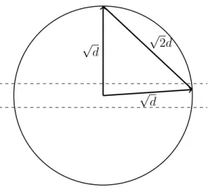
Calculation of width of the annulus
We now show that most of the mass of the Gaussian is within an annulus of constant width and radius √d−1. The probability mass of the Gaussian as a function of r is g(r) =rd−1e−r2/2. To determine the width of the annulus in which g(r) is nonnegligible, consider the logarithm ofg(r)
f(r) = lng(r) = (d−1) lnr− r
2
2. Differentiatingf(r),
f0(r) = d−1
r −r and f
00
(r) = −d−1
r2 −1≤ −1.
Note that f0(r) = 0 at r = √d−1 and f00(r)< 0 for all r. The Taylor series expansion forf(r) about √d−1, is
f(r) = f(√d−1) +f0(√d−1)(r−√d−1) + 1 2f
00
(√d−1)(r−√d−1)2+· · · . Thus,
f(r) =f(√d−1) +f0(√d−1)(r−√d−1) + 1 2f
00
(ζ)(r−√d−1)2
for some pointζ between√d−1 and r.1 Since f0(√d−1) = 0, the second term vanishes
and
f(r) = f(√d−1) + 1 2f
00
(ζ)(r−√d−1)2. Since the second derivative is always less than−1,
f(r)≤f(√d−1)− 1
2(r−
√
d−1)2. Recall that g(r) =ef(r). Thus
g(r)≤ef(
√
d−1)−12(r−√d−1)2
=g(√d−1)e−12(r−
√
d−1)2
.
Letcbe a positive real and letI be the interval [√d−1−c,√d−1 +c]. We calculate the ratio of an upper bound on the probability mass outside the interval to a lower bound on the total probability mass. The probability mass outside the intervalI is upper bounded by
Z
r /∈I
g(r)dr ≤ Z
√
d−1−c r=0
g(√d−1)e−(r−
√
d−1)2/2
dr+
Z ∞
r=√d−1+c
g(√d−1)e−(r−
√
d−1)2/2
dr
≤2g(√d−1)
Z ∞
r=√d−1+c
e−(r−
√
d−1)2/2
dr = 2g(√d−1)
Z ∞
y=c
e−y2/2 dy
≤2g(√d−1)
Z ∞
y=c
y ce
−y2/2
dy = 2
cg(
√
d−1)e−c2/2.
To get a lower bound on the probability mass in the interval [√d−1−c,√d−1 +c], consider the subinterval [√d−1,√d−1+2c].Forrin the subinterval [√d−1,√d−1+2c], f00(r)≥ −2 and
f(r)≥f(√d−1)−(r−√d−1 )2 ≥f(√d−1)− c
2
4. Thus
g(r) =ef(r)≥ef
√
d−1
e−c
2 4 =g(
√
d−1)ec42.
Hence, R
√
d−1+c
2
√
d−1 g(r) dr ≥
c
2g(
√
d−1)e−c2/4
and the fraction of the mass outside the interval is
2
cg( √
d−1)e−c2/2
c
2g(
√
d−1)e−c2/4
+2cg(√d−1)e−c2/2 =
2
c2e
−c2
4
c
2 +
2
c2e
−c2 4
= e
−c2
4
c2
4 +e −c2
4
≤ 4
c2e −c2
4 .
This establishes the following lemma.
Lemma 1.8 For a d-dimensional spherical Gaussian of variance 1, all but c42e
−c2/4
frac-tion of its mass is within the annulus √d−1−c≤r≤√d−1 +c for any c >0.
Separating Gaussians
Gaussians are often used to model data. A common stochastic model is the mixture model where one hypothesizes that the data is generated from a convex combination of simple probability densities. An example is two Gaussian densitiesF1(x) andF2(x) where
data is drawn from the mixture F(x) =w1F1(x) +w2F2(x) with positive weightsw1 and
√
d
√
d
√
2d
Figure 1.12: Two randomly chosen points in high dimension are almost surely nearly orthogonal.
means are very close, then given data from the mixture, one cannot tell for each data point whether it came from F1 or F2. The question arises as to how much separation is
needed between the means to tell which Gaussian generated which data point. We will see that a separation of Ω(d1/4) suffices. Later, we will see that with more sophisticated
algorithms, even a separation of Ω(1) suffices.
Consider two spherical unit variance Gaussians. From Lemma 1.8, most of the prob-ability mass of each Gaussian lies on an annulus of width O(1) at radius √d−1. Also e−|x|2/2factors intoQ
ie
−x2
i/2and almost all of the mass is within the slab{x|−c≤x
1 ≤c},
for c∈O(1). Pick a point x from the first Gaussian. After picking x, rotate the coordi-nate system to make the first axis point towards x. Then, independently pick a second pointyalso from the first Gaussian. The fact that almost all of the mass of the Gaussian is within the slab {x| −c ≤ x1 ≤ c, c ∈ O(1)} at the equator says that y’s component
along x’s direction is O(1) with high probability. Thus, y is nearly perpendicular to x. So, |x−y| ≈p|x|2+|y|2. See Figure 1.12. More precisely, since the coordinate system
has been rotated so that x is at the North Pole, x = (p(d)±O(1),0, . . .). Since y is almost on the equator, further rotate the coordinate system so that the component of y that is perpendicular to the axis of the North Pole is in the second coordinate. Then y= (O(1),p(d)±O(1), . . .). Thus,
(x−y)2 =d±O(√d) +d±O(√d) = 2d±O(√d) and |x−y|=p(2d)±O(1).
Given two spherical unit variance Gaussians with centers p and q separated by a distanceδ, the distance between a randomly chosen pointxfrom the first Gaussian and a randomly chosen pointyfrom the second is close to√δ2+ 2d, sincex−p,p−q,andq−y
√
d
δ
p q
x z
y
√
δ2+ 2d
δ √2d
Figure 1.13: Distance between a pair of random points from two different unit spheres approximating the annuli of two Gaussians.
are nearly mutually perpendicular. To see this, pickx and rotate the coordinate system so thatx is at the North Pole. Let z be the North Pole of the sphere approximating the second Gaussian. Now pick y. Most of the mass of the second Gaussian is within O(1) of the equator perpendicular to q−z. Also, most of the mass of each Gaussian is within distanceO(1) of the respective equators perpendicular to the line q−p. Thus,
|x−y|2 ≈δ2+|z−q|2+|q−y|2
=δ2+ 2d±O(
√
d)).
To ensure that the distance between two points picked from the same Gaussian are closer to each other than two points picked from different Gaussians requires that the upper limit of the distance between a pair of points from the same Gaussian is at most the lower limit of distance between points from different Gaussians. This requires that
√
2d+O(1) ≤√2d+δ2−O(1) or 2d+O(√d)≤2d+δ2, which holds when δ ∈Ω(d1/4).
Thus, mixtures of spherical Gaussians can be separated provided their centers are sepa-rated by more thand14. One can actually separate Gaussians where the centers are much
closer. In Chapter 4, we will see an algorithm that separates a mixture of k spherical Gaussians whose centers are much closer.
Algorithm for separating points from two Gaussians
Calculate all pairwise distances between points. The cluster of smallest pairwise distances must come from a single Gaussian. Remove these points and repeat the process.
Given a set of sample points, x1,x2, . . . ,xn, in a d-dimensional space, we wish to find the spherical Gaussian that best fits the points. Let F be the unknown Gaussian with mean µ and variance σ2 in every direction. The probability of picking these very points
when sampling according toF is given by
cexp − (x1 −µ)
2
+ (x2−µ)2+· · ·+ (xn−µ)2 2σ2
!
where the normalizing constant c is the reciprocal of
R
e−
|x−µ|2
2σ2 dx n
. In integrating from
−∞to∞,one could shift the origin toµand thuscis
R
e− |x|2
2σ2dx
−n
and is independent of µ.
The Maximum Likelihood Estimator (MLE) ofF, given the samplesx1,x2, . . . ,xn, is the F that maximizes the above probability.
Lemma 1.9 Let {x1,x2, . . . ,xn} be a set of n points in d-space. Then (x1−µ)2 +
(x2−µ)2+· · ·+(xn−µ)2 is minimized whenµis the centroid of the pointsx1,x2, . . . ,xn,
namely µ= n1(x1+x2+· · ·+xn).
Proof: Setting the derivative of (x1−µ)2+ (x2−µ)2+· · ·+ (xn−µ)2 to zero yields −2 (x1−µ)−2 (x2−µ)− · · · −2 (xd−µ) = 0.
Solving forµ gives µ= n1(x1+x2+· · ·+xn).
In the maximum likelihood estimate for F, µ is set to the centroid. Next we show that σ is set to the standard deviation of the sample. Substitute ν = 2σ12 and a =
(x1−µ)2+ (x2−µ)2+· · ·+ (xn−µ)2 into the formula for the probability of picking the
pointsx1,x2, . . . ,xn. This gives
e−aν
R
x
e−|x|2ν
dx
n.
Now,a is fixed and ν is to be determined. Taking logs, the expression to maximize is
−aν−nln
Z
x
e−ν|x|2dx
.
To find the maximum, differentiate with respect toν, set the derivative to zero, and solve forσ. The derivative is
−a+n
R
x
|x|2e−ν|x|2
dx
R
x
e−ν|x|2
Settingy=√νx in the derivative, yields
−a+ n ν
R
y
y2e−y2
dy
R
y e−y2
dy .
Since the ratio of the two integrals is the expected distance squared of a d-dimensional spherical Gaussian of standard deviation √1
2 to its center, and this is known to be
d
2, we
get −a+ nd2ν. Substituting σ2 for 1
2ν gives −a+ndσ
2. Setting−a+ndσ2 = 0 shows that
the maximum occurs when σ =
√
a
√
nd. Note that this quantity is the square root of the
average coordinate distance squared of the samples to their mean, which is the standard deviation of the sample. Thus, we get the following lemma.
Lemma 1.10 The maximum likelihood spherical Gaussian for a set of samples is the one with center equal to the sample mean and standard deviation equal to the standard deviation of the sample.
Let x1,x2, . . . ,xn be a sample of points generated by a Gaussian probability
distri-bution. µ = 1n(x1 +x2+· · ·+xn) is an unbiased estimator of the expected value of
the distribution. However, if in estimating the variance from the sample set, we use the estimate of the expected value rather than the true expected value, we will not get an unbiased estimate of the variance since the sample mean is not independent of the sam-ple set. One should useµ = n−11 (x1+x2+· · ·+xn) when estimating the variance. See
appendix.
1.7
Random Projection and the Johnson-Lindenstrauss
Theo-rem
Many high-dimensional problems such as the nearest neighbor problem can be sped up by projecting the data to a random lower-dimensional subspace and solving the problem there. This technique requires that the projected distances have the same ordering as the original distances. If one chooses a random k-dimensional subspace, then indeed all the projected distances in the k-dimensional space are approximately within a known scale factor of the distances in the d-dimensional space. We first show that for one distance pair, the probability of its projection being badly represented is exponentially small ink. Then we use the union bound to argue that failure does not happen for any pair.
Project a fixed (not random) unit length vector v in d-dimensional space onto a randomk-dimensional space. By the Pythagoras theorem, the length squared of a vector is the sum of the squares of its components. Thus, we would expect the squared length of the projection to be kd. The following theorem asserts that the squared length of the projection is very close to this quantity.
Theorem 1.11 (The Random Projection Theorem): Let v be a fixed unit length vector in a d-dimensional space and let W be a random k-dimensional subspace. Let w be the projection of v onto W. For any 0≤ε≤1, Prob |w|2− k
d ≥εkd
≤4e−kε
2 64 .
Proof: A random subspace is generated by selecting a set of basis vectors. Working with such a set of dependent vectors is difficult. However, projecting a fixed vector onto a random subspace is the same as projecting a random vector onto a fixed subspace. That is, the probability distribution of w in the theorem is the same as the probability dis-tribution of the vector obtained by taking a random unit length vector z and projecting it onto the fixed subspace U spanned by its first k coordinate vectors. This is because one can rotate the coordinate system so that a set of basis vectors for W are the first k coordinate axes.
Let ˜z be the projection of z onto U. We will prove that |˜z|2 ≈ k
d. Now
|˜z|2− k d is
greater than or equal to εkd if either |˜z|2 ≤ (1−ε)kd or |˜z|2 ≥ (1−ε)kd. Let β = 1−ε. We will prove that Prob |˜z|2 < βkd≤2e− kε
2
4 . The other case is similar and is omitted.
Together they imply Prob |w|2− k d ≥εkd
≤4e−kε
2 64 .
Pick a random vector z of length one by picking independent Gaussian random vari-ables x1, x2, . . . , xd, each with mean zero and variance one. Let x= (x1, x2, . . . , xd) and
take z=x/|x|. This yields a random vector z of length one. Prob
|˜z|2 < βk d
=P rob
|˜z|2 ≤βk
d|z|
2
= Prob
x21 +x22+· · ·+x2k < βk d x
2 1+x
2
2+· · ·+x 2
d
= Probβk x21+x22+· · ·+x2d−d x21+x22+· · ·+x2k>0. If kε2 <64, then 4e−kε
2
64 >1, so the probability upper bound asserted in the theorem is
greater than one and there is nothing to prove. So assume that kε2 ≥ 64 which implies
ε≥ √8
k. Definec=ε √
k/4 and since ε≥ √8
k, it follows that c≥2.
Now if βk(x2
1+x22+· · ·+x2d)−d(x21+x22+· · ·+x2k)>0, then one of the following
inequalities must hold withc=ε√k/4:
βk(x21+x22+· · ·+x2d)> βk(√d−1 +c)2 (1.6) d(x21+x22+· · ·+x2k)< βk(√d−1 +c)2. (1.7) Using Lemma 1.8 we will prove that the probability of each of (1.6) and (1.7) is at most
4
c2e
−c2
4 = 64
kε2e
−kε2
64 ≤e−kε 2/64
so that the probability of at least one of (1.6) or (1.7) is less than or equal to 2e−kε
2
64 which proves the theorem. Lemma 1.8 implies
with probability less than or equal to c42e
−c2/4 ≤ e−kε2/64 from which (1.6) follows. For
(1.7), from Lemma 1.8,
Prob(d(x21+x22+· · ·+x2k)< d(√k−1−c)2) with probability less than or equal to c42e
−c2/4
≤e−kε2/64. Since βk < d, βk(√d−1−c)2 ≤d(√k−1−c)2 and thus
Probd(x21+x22 +· · ·+x2k)< βk(√d−1−c)2
≤Probd(x21+x22+· · ·+x2k)< d(√k−1−c)2
≤e−kε2/64
completing the proof of Theorem 1.11.
The Random Projection Theorem enables us to argue, using the union bound, that the projection to order logn dimensions preserves all relative pairwise distances between a set of n points. This is the content of the Johnson-Lindenstrauss Lemma.
Theorem 1.12 (Johnson-Lindenstrauss Lemma): For any 0< ε <1 and any inte-gern, let k be an integer such that
k ≥ 64 lnn
ε2 .
For any set P of n points in Rd, a random projection f mapping f : Rd → Rk has the
property that for all u and v in P, (1−ε)k
d|u−v|
2 ≤ |
f(u)−f(v)|2 ≤(1 +ε)k
d|u−v|
2
with probability at least 9/10.
Proof: Let S be a random k-dimensional subspace and let f(u) be the projection of u ontoS multiplied by the scalar
q d
k. Applying the Random Projection Theorem 1.11, for
any fixedu and v, the probability that kf(u)−f(v)k2 is outside the range
h
(1−ε)βk|u−v|2,(1 +ε)k
β|u−v|
2i
is at most
e− kε
2
16 =e−4 lnn = 1
n4.
By the union bound the probability that any pair has a large distortion is less than
n
2
× 1
n4 ≤
1
Remark: It is important to note that the conclusion of Theorem 1.12 is asserted for all u and v in P, not just for most u and v. The weaker assertion for most u and v is not that useful, since we do not know whichvwould end up being the closest point to u and an assertion for most may not cover the particularv. A remarkable aspect of the theorem is that the number of dimensions in the projection is only dependent logarithmically on n. Since k is often much less than d, this is called a dimension reduction technique.
For the nearest neighbor problem, if the database has n1 points and n2 queries are
expected during the lifetime, then taken=n1+n2 and project the database to a random
k-dimensional space, where k ≥ 64 lnn
ε2 . On receiving a query, project the query to the
same subspace and compute nearby database points. The theorem says that this will yield the right answer whatever the query with high probability. Note that the exponentially small in k probability in Theorem 1.11 was useful here in making k only dependent on logn, rather thann.
1.8
Bibliographic Notes
The word vector model was introduced by Salton [?]. Taylor series remainder mate-rial can be found in Whittaker and Watson 1990, pp. 95-96. There is vast literature on Gaussian distribution, its properties, drawing samples according to it, etc. The reader can choose the level and depth according to his/her background. For Chernoff bounds and their applications, see [?] or [?]. The proof here and the application to heavy-tailed distributions is simplified from [?]. The original proof of the Random Projection Theo-rem by Johnson and Lindenstrauss was complicated. Several authors used Gaussians to simplify the proof, see [?] for details and applications of the theorem. The proof here is due to Das Gupta and Gupta [?].
The SVD based algorithm for identifying the space spanned by centers of spherical Gaus-sians is from Vempala and Wang [?]. The paper handles more complex densities besides spherical Gaussians, but the restricted case of spherical Gaussians contains the key ideas.
1.9
Exercises
Exercise 1.1 Assume you have 100 million documents each represented by a vector in the word vector model. How would you represent the documents so that given a query with a small number of words you could efficiently find the documents with the highest dot product with the query vector? Given the number of documents you do not have time to look at every document.
Exercise 1.2 Let x and y be independent random variables with uniform distribution in [0,1]. What is the expected value E(x)? E(x2)? E(x−y)? E(xy)? and E((x−y)2)? Exercise 1.3 What is the distribution of the distance between two points chosen uni-formly at random in the interval [0,1]? In the unit square? In the unit cube in 100 dimensions? Give a qualitative answer.
Exercise 1.4 What is the expected distance between two points selected at random inside a d-dimensional unit cube? For two points selected at random inside a d-dimensional unit sphere? What is the cosine of the angle between them?
Exercise 1.5 Consider two random 0-1 vectors in high dimension. What is the angle between them? What is the probability that the angle is less than 45?
Exercise 1.6 Place two unit-radius spheres in d-dimensions, one at (-2,0,0,. . . ,0 ) and the other at (2,0,0,. . . ,0). Give an upper bound on the probability that a random line through the origin will intersect the spheres.
Exercise 1.7 Generate a 1,000 points at vertices of a 1,000-dimensional cube. Select two points iand j at random and find a path fromi toj by the following algorithm. Start at i and go to a pointk differing fromiin only one coordinate so thatdist(i, k)and dist(j, k) are both less than dist(i, j). Then continue the path by the same algorithm from k to j. What is the expected length of the path?
Exercise 1.8 (Overlap of spheres)Let x be a random sample from the unit sphere in d-dimensions with the origin as center.
1. What is the mean of the random variable x? The mean, denotedE(x), is the vector, whose ith component is E(x
i).
2. What is the component-wise variance of x?
3. Show that for any unit length vector u, the variance of the real-valued random vari-able uT ·x is Pd
i=1
u2
iE(x2i). Using this, compute the variance and standard deviation
4. Given two spheres in d-space, both of radius one whose centers are distance aapart, show that the volume of their intersection is at most
4e−a2(d8−1)
a√d−1 times the volume of each sphere.
Hint: Relate the volume of the intersection to the volume of a cap, then, use Lemma 1.2.
5. From (4), conclude that if the inter-center separation of the two spheres of radius r is Ω(r/√d), then they share very small mass. Theoretically, at this separation, given randomly generated points from the two distributions, one inside each sphere, it is possible to tell which sphere contains which point, i.e., classify them into two clusters so that each cluster is exactly the set of points generated from one sphere. The actual classification requires an efficient algorithm to achive this. Note that the inter-center separation required here goes to zero as d gets larger, provided the radius of the spheres remains the same. So, it is easier to tell apart spheres (of the same radii) in higher dimensions.
Exercise 1.9 Derive an upper bound on Rx∞=αe−x2
dx where α is a positive real. Discuss for what values ofα this is a good bound.
Hint: Use e−x2 ≤ x αe
−x2
for x≥α.
Exercise 1.10 What is the formula for the incremental unit of area in using polar coor-dinates to integrate the area of a circle that lies in a 2-dimensional cone whose vertex is at the center of the circle? What is the formula for the integral? What is the value of the integral if the cone is36◦?
Exercise 1.11 For what value of d is the volume, V(d), of a d-dimensional unit sphere maximum?
Hint: Consider the ratio VV(d(−1)d) for odd and even values ofd.
Exercise 1.12 How does the volume of a sphere of radius two behave as the dimension of the space increases? What if the radius was larger than two but a constant independent of d? What function of d would the radius need to be for a sphere of radius r to have approximately constant volume as the dimension increases?
Exercise 1.13
1. What is the volume of a sphere of radius r in d-dimensions? 2. What is the surface area of a sphere of radius r in d-dimensions?
3. What is the relationship between the volume and the surface area of a sphere of radius r in d-dimensions?
4. Why does the relationship determined in (3) hold?
Exercise 1.14 Consider vertices of a d-dimensional cube of width two centered at the origin. Vertices are the points(±1,±1, . . . ,±1). Place a unit-radius sphere at each vertex. Each sphere fits in a cube of width two and, thus, no two spheres intersect. Show that the probability that a point of the cube picked at random will fall into one of the2d unit-radius
spheres, centered at the vertices of the cube, goes to 0 as d tends to infinity. Exercise 1.15 Consider the power law probability density
p(x) = c Max(1, x2)
over the nonnegative real line. 1. Determine the constant c.
2. For a nonnegative random variable x with this density, does E(x) exist? How about E(x2)?
Exercise 1.16 Consider d-space and the following density over the positive orthant: p(x) = c
Max(1,|x|α).
Show thatα > dis necessary for this to be a proper density function. Show that α > d+ 1 is a necessary condition for a (vector-valued) random variable xwith this density to have an expected value E(|x|). What condition do you need if we want E(|x|2) to exist?
Exercise 1.17 Consider the upper hemisphere of a unit-radius sphere in d-dimensions. What is the height of the maximum volume cylinder that can be placed entirely inside the hemisphere? As you increase the height of the cylinder, you need to reduce the cylinder’s radius so that it will lie entirely within the hemisphere.
Exercise 1.18 What is the volume of a radius r cylinder of height h in d-dimensions? Exercise 1.19 For a 1,000-dimensional unit-radius sphere centered at the origin, what fraction of the volume of the upper hemisphere is above the plane x1 = 0.1? Above the
plane x1 = 0.01?
Exercise 1.20 Almost all of the volume of a sphere in high dimensions lies in a narrow slice of the sphere at the equator. However, the narrow slice is determined by the point on the surface of the sphere that is designated the North Pole. Explain how this can be true if several different locations are selected for the North Pole.
Exercise 1.21 Explain how the volume of a sphere in high dimensions can simultaneously be in a narrow slice at the equator and also be concentrated in a narrow annulus at the surface of the sphere.
Exercise 1.22 How large mustε be for 99% of the volume of ad-dimensional unit-radius sphere to lie in the shell of ε-thickness at the surface of the sphere?
Exercise 1.23
1. Write a computer program that generates n points uniformly distributed over the surface of a unit-radius d-dimensional sphere.
2. Generate 200 points on the surface of a sphere in 50 dimensions.
3. Create several random lines through the origin and project the points onto each line. Plot the distribution of points on each line.
4. What does your result from (3) say about the surface area of the sphere in relation to the lines, i.e., where is the surface area concentrated relative to each line? Exercise 1.24 If one generates points in d-dimensions with each coordinate a unit vari-ance Gaussian, the points will approximately lie on the surface of a sphere of radius √d. What is the distribution when the points are projected onto a random line through the origin?
Exercise 1.25 Project the surface area of a sphere of radius √d in d-dimensions onto a line through the center. For d equal 2 and 3, derive an explicit formula for how the projected surface area changes as we move along the line. For larged, argue (intuitively) that the projected surface area should behave like a Gaussian.
Exercise 1.26 Generate 500 points uniformly at random on the surface of a unit-radius sphere in 50 dimensions. Then randomly generate five additional points. For each of the five new points calculate a narrow band at the equator assuming the point was the North Pole. How many of the 500 points are in each band corresponding to one of the five equators? How many of the points are in all five bands?
Exercise 1.27 We have claimed that a randomly generated point on a sphere lies near the equator of the sphere independent of the point selected for the North Pole. Is the same claim true for a randomly generated point on a cube? To test this claim, randomly generate ten ±1 valued vectors in 128 dimensions. Think of these ten vectors as ten choices for the North Pole. Then generate some additional ±1 valued vectors. To how many of the original vectors is each of the new vectors close to being perpendicular, that is how many of the equators is each new vectors close to.
Exercise 1.28 Consider a slice of a 100-dimensional sphere that lies between two parallel planes each equidistant from the equator and perpendicular to the line from the North to South Pole. What percentage of the distance from the center of the sphere to the poles must the planes be to contain 95% of the surface area?