www.scholink.org/ojs/index.php/jetss
Original Paper
Language Recognition Method of Convolutional Neural
Network Based on Spectrogram
Wu Min1* & Zhu Shanshan1 1
Information Engineering University Luoyang Campus, Language Information Processing, Luoyang City, Henan Province, 471000, China
*
Wu Min, Information Engineering University Luoyang Campus, Language Information Processing, Luoyang City, Henan Province, 471000, China
Received: March 18, 2019 Accepted: April 27, 2019 Online Published: December 30, 2019 doi:10.22158/jetss.v1n2p113 URL: http://dx.doi.org/10.22158/jetss.v1n2p113
Abstract
Language recognition is an important branch of speech technology. As a front -end technology of speech information processing, higher recognition accuracy is required. It is found through research that there are obvious differences between the language maps of different languages, which can be used for language identification. This paper uses a convolutional neural network as a classification model, and compares the language recognition effects of traditional language recognition features and spectrogram features on the five language recognition tasks of Chinese, Japanese, Vietnamese, Russian, and Spanish through experiments. The best effect is the ivector feature, and the spectrogram feature has a higher F value than the low -dimensional ivector feature.
Keywords
language recognition, CNN, spectrogram
1. Introduction
Language is a form of communication between people, and people cannot communicate with each other without language. Although people’s thoughts can be transmitted through pictures, actions, expressions, etc., language is the most important and convenient medium. Language is the most convenient and fastest way for humans to exchange information, and speech is the acoustic expression of language. Voice communication is the most natural way for human beings, and it is also the basic means of communication for human beings today (Yang, 1995; He, 2002).
regions using different languages has become increasingly active (Ye, 2000). In the past, speech recognition for specific languages was moving towards multilingual speech recognition, and language recognition was precisely distinguished by computers. Best means of language kind. Language recognition, that is, the automatic language recognition technology of speech, specifically refers to the technology that automatically recognizes the language type of the input speech signal. Language recognition technology has an irreplaceable role in practical applications. For example, in the field of national security and defense, the worldwide communication and consulting materials that can be obtained are often composed of voice signals in multiple languages in different regions. Language recognition technology can be used as the front-end technology of speech recognition technology. The speech signals of a specific language are screened and then processed for speech-to-text recognition. With the continuous progress of various information acquisition methods, the information obtained has become more, easier and more redundant, as has the voice information. With the emergence of more and more multilingual voice environments, the elimination of all redundant information in non-target languages in voice information has become more critical, and the need for language recognition for voice has become greater and greater.
This paper attempts to combine deep learning methods to build a convolutional neural network classification model, and recognizes by using different language recognition features, including traditional language recognition features: MFCC, ivector, and spectrogram features. By comparing the recognition effects of different features in the language, the language recognition features with better recognition effect are explored.
2. Spectral Features
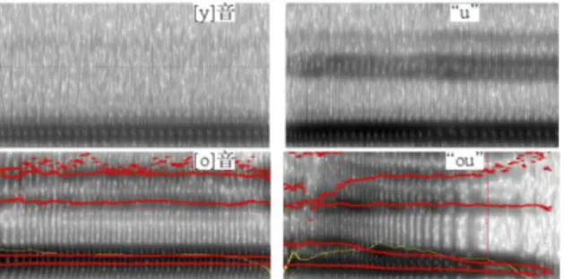
By consulting relevant data, it is found that there are many different differences in pronunciation between different languages. Studies on pronunciation and phonetics have shown that the different sound quality of vowels depends on changes in the shape of the mouth. The changes in the shape of the oral cavity are mainly caused by the forward and backward movement of the tongue, and the stretching or rounding of the lips. The obvious differences in the pronunciation of various languages are the different pronunciation of phonemes and the number of phonemes. As shown in Figure 1, the similar pronunciation in Chinese and Russian has obvious differences in the grammar. The pure vowel “y” in Russian pronunciation and the Chinese pinyin “u” have more rounded lips when pronounced. It is more tense and has smaller openings. The pinyin “u” has obvious three voiced formants on the spectrogram. The Russian vowel “y” does not have (Zhao, 2012). Many vowels in Russian need to retract and raise the tongue, and include many tongue rolls. In addition, there are tremolos in consonants. These are the characteristics of Russian speech. These characteristics are made by the vocal organ different (Zhang, 2014; Chen, 2017).
Figure 1. Comparison of Chinese Phonetic Notation “u” “ou” and Russian Vowel “y” “o”
The sonogram contains obvious features of language identification, so this article attempts to compare it with traditional language identification features. At the same time, the convolutional neural network in the deep neural network was selected as the classification model, and the convolutional neural network was used as a model for the remarkable effect of picture recognition. In theory, it can better identify the differences in the spectrum maps between different languages.
3. Traditional Language Recognition Features
In this paper, two traditional language recognition features MFCC and ivector are selected for experiments to try to verify the efficient recognition performance of ivector and compare the performance differences between traditional features. Among them, MFCC is a relatively popular recognition feature in the early stage. As a characteristic parameter that simulates the auditory characteristics of the human ear, it has achieved good recognition results in early speech recognition, language recognition, and voiceprint recognition tasks. This feature is modeled by mathematical methods to obtain low-dimensional high-density specific features of speech, and has achieved excellent results in various tasks of speech processing.
3.1 MFCC
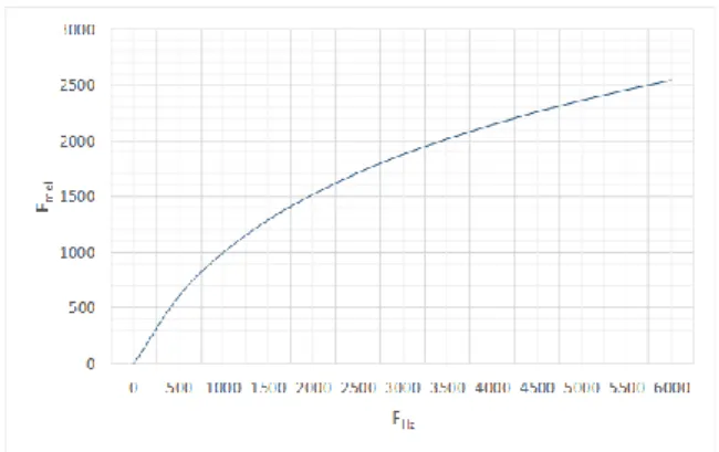
The hearing sensitivity of the human ear to speech signals in different frequency ranges is very different. It has a non-linear characteristic, that is, there is a non-linearity between the frequency of the speech signal that the human ear can sense and the actual frequency of the speech signal. Mapping relations. After specific experimental research, for speech signals with a frequency below 1 kHz, the human ear’s hearing ability is linear with the actual signal frequency; for speech signals with a frequency range above 1 kHz, the two are no longer a linear relationship. It is more similar to a logarithmic relationship. In other words, people are more sensitive to the high-frequency part of the speech signal. In view of the above human ear hearing characteristics, a Mel frequency cepstrum parameter based on Mel scale transformation is proposed, and defining a Mel scale is equivalent to One-thousandth of the perception of a 1kHz tone. The corresponding relationship is shown in Figure 2. Mel frequency expresses the relationship from linear frequency to perceived frequency to conversion. The calculation formula is as follows:
𝑚𝑒𝑙(𝑓) = 2595 ∗ 𝑙𝑔(1 + 𝑓
700) (1)
According to further research, the hearing of the human ear has a masking effect, that is, it is impossible to effectively distinguish all frequency components of the speech signal. When the frequency of the two speech tones is close, the human ear can only perceive one of the tones and cannot distinguish These two tones of different frequencies. In order for the human ear to be able to distinguish between two different frequency tones, it is necessary to ensure that the frequency of the two tones heard by the human ear needs a certain frequency band range. This frequency band is the critical band, and its corresponding bandwidth is the critical bandwidth. The growth trend of critical bandwidth and perceived frequency is basically the same: that is, when the frequency is lower than 1 kHz, the critical bandwidth is approximately linearly increased, and when it is higher than 1 kHz, it is approximately logarithmic. Therefore, in practical applications, a triangular filter is often used to construct a critical filter bank, which is a so-called Mel filter bank.
Figure 2. Relationship between Mel Frequency and Linear Frequency
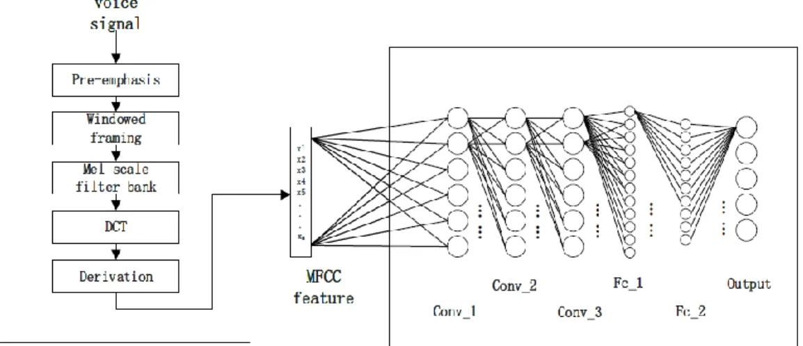
The specific steps of obtaining Mel frequency cepstrum coefficients can be divided into four steps: first, the original speech signal is sampled and quantized, and windowed and framed, etc., to obtain the speech sequence of each frame speech signal; Perform a fast Fourier transform to get its frequency spectrum, and then square its frequency spectrum to get its amplitude spectrum. The third step is to pass the amplitude spectrum through the Mel frequency filter bank (usually 12 to 16) to get its output parameters. In the last step, energy calculation is performed on the parameters obtained in the previous step, and then the discrete cosine transform is performed to obtain the Mel frequency cepstrum parameters. In order to obtain the dynamic characteristics of the spectral parameters, the first-order second-order difference calculation of the obtained Mel frequency cepstrum coefficient parameters is often performed. The first-order second-order parameters and the original parameters together constitute a 36-48-dimensional feature. Features perform better in speech recognition, voiceprint recognition, and language recognition.
Mel frequency cepstrum parameter characteristic parameters. Because the Mel frequency scale can enhance the low-frequency details of the speech signal, and the human voice is often low-frequency,
the low-frequency part of the speech signal contains a lot of useful information. Therefore, the Mel frequency is based on the Mel frequency. The scaled Mel frequency cepstrum parameter can better highlight the useful part of the speech signal. In addition, no modeling is required to obtain Mel frequency cepstrum parameters, and its application range is wider. And in the solution process, it has a significant promotion effect on speech segmentation, speech synthesis and endpoint detection of speech signals. A large number of studies have shown that the application effect of MFCC features in language recognition is also very good.
3.2 Ivector
ivector is proposed to improve the GMM Supervector (GSV). The GSV-SVM method is representative of typical statistical language recognition methods. The average supervector obtained after modeling a Gaussian mixture model is used as a recognition feature, and low-dimensional acoustic features are mapped to a high-dimensional GMM space to obtain more effective features and improve The recognition performance is improved, but at the same time, because of its large feature dimension, it brings huge computational overhead to the recognition part of the backend (Yang, 2015). In addition, in a complex environment, the GSV calculation process did not suppress the effects of various noises, which led to a significant reduction in its recognition performance. In recent years, due to the rise of subspace research, techniques such as Factor Analysis (FA) have been derived to map the Gaussian mean supervector space to obtain a low-dimensional vector that maximizes the language discriminative information in this space. And use this vector as a feature to perform language recognition. The principle of the ivector algorithm is similar. The features it extracts not only greatly reduce the feature dimension compared to GSV, reduce the complexity of the operation, but also effectively suppress the interference of non-relevant information such as noise. ivector has become the main feature of current language recognition non-deep learning methods (Yang, Qu, & Zhang, 2014)。
The core model of the ivector algorithm is as follows. By analyzing the average supervector of the Gaussian mixture model, the model considers that the average supervector of the Gaussian mixture model for a specific speech is composed of two parts:
𝑀(𝑥) = 𝑚 + 𝑇𝑤(𝑥)
(2)𝑀(𝑥) represents a Gaussian mixture model mean supervector of speech segment x that is related to language and channel, m represents a language and channel independent mean supervector, and T is a global space transformation matrix, which is an expansion from A matrix composed of N bases in the total variable space, 𝑤(𝑥) is a hidden variable that obeys the normal distribution, and is called the global space difference factor. The significance of this model is that any speech segment x can be represented as the superposition of the inter-class differences, language, and channel-independent mean supervectors that constitute the speech segment x through 𝑇𝑤(𝑥). And ivector is actually an estimate of 𝑤(𝑥).
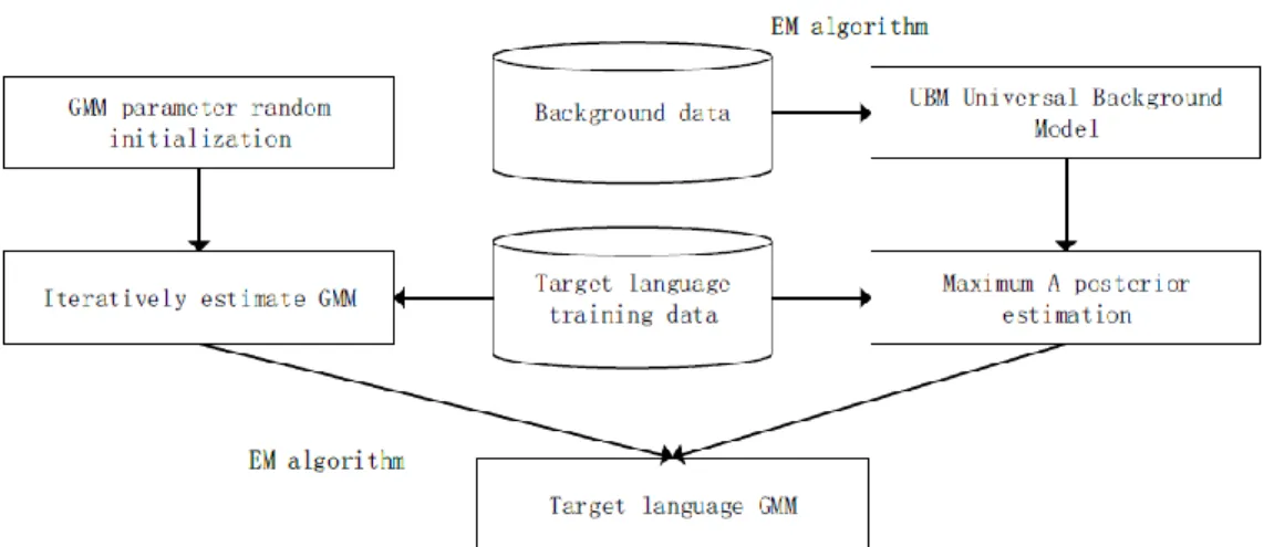
The calculation of ivector can also be implemented using the expectation maximization algorithm. The general process is divided into three steps. The first step is to obtain a universal Gaussian mixture
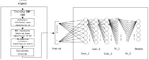
model-Universal Background Model (UBM). The second step uses the expectation maximization algorithm to repeat. Iteratively obtain the global space transformation matrix T. The third step is to extract the ivector. When the global space transformation matrix is calculated and the average supervector of the input speech is calculated, the maximum vector posterior point estimate of the global spatial difference factor is calculated to obtain the ivector feature vector representing the speech segment.
The specific process is as follows:
Step 1 First, a Gaussian mixture model is trained by using an expectation maximization algorithm on a part of speech corpora that includes all languages, which is a general background model. The training process is shown in Figure 3. The GMM-UBM has C Gaussian components, and the parameters of the c-th single Gaussian model can be expressed as:
𝜆𝑐= (𝜋𝑐, 𝜇𝑐, 𝛴𝑐), 𝑐 ∈ 𝐶 (3)
Among them, the three parameters represent the Gaussian mixture weight, the mean vector, and the covariance matrix, and a complete GMM can be represented by these parameters.
Step 2 Directly extract the mean vector of each single Gaussian model and splice it into a new vector. Assuming that the acoustic feature dimension of each frame of speech is D, then the obtained 𝐶 ⋅ 𝐷
mean supervector is the pending 𝑚.
Step 3 According to the GMM-UBM, a maximum posterior probability (Maximum A Posterior, MAP) calculation method is used to obtain the average supervector of the training speech input, which is
𝑀(𝑥) in the expression.
Figure 3. GMM-UBM Model Training Process Diagram
Step 4 Calculate sufficient statistics for the s-segment training speech of each single Gaussian model. The following statistics will be used multiple times in the following. It is assumed that the s-segment speech has 𝐻(𝑠) frames and the s-segment speech is acoustic. The feature is 𝑋(𝑠), and the acoustic
feature vector of each frame is expanded as 𝑥𝑖, 𝑖 ∈ 𝐻(𝑠): Zero-order statistics: 𝑁𝑐(𝑠) = ∑ 𝑖=1 𝐻(𝑠) 𝑃𝜆(𝑐|𝑥𝑖) (4) First-order statistics: 𝐹𝑐(𝑠) = ∑ 𝑖=1 𝐻(𝑠) 𝑃𝜆(𝑐|𝑥𝑖)(𝑥𝑖− 𝜇𝑖) (5)
Where 𝑃𝜆(𝑐|𝑥𝑖) is the posterior probability of the c-th Gaussian component, the calculation formula is as follows:
𝑃𝜆(𝑐|𝑥𝑖) =
𝑤𝑖𝑝𝑖(𝑥𝑖)
∑𝑗=1𝑀 𝑤
𝑗𝑝𝑗(𝑥𝑖) (6)
𝑥𝑖 is the acoustic feature of the i-th frame of a sentence, and the 𝑥𝑖 in the original formula was changed to (𝑥𝑖− 𝜇𝑖) when calculating the first-order statistics, because the latter achieved the decentralization effect by subtracting the mean Compared with the former, the latter is more prominent in language characteristics. Combining sufficient statistics for all Gaussian components of the speech segment yields: 𝑁(𝑠) = [ 𝑁1(𝑠)𝐼 0 . . . 0 𝑁𝑐(𝑠)𝐼 ] (7) 𝐹(𝑠) = [ 𝐹1(𝑠) . . . 𝐹𝑐(𝑠) ] (8)
Next, use the EM algorithm to derive the T matrix. First, calculate the expected E step: The Q function of the i-th iteration is as follows:
𝑄(𝑇|𝑇(𝑖)) = ∑ 𝑠=1 𝑆 𝐸(𝑙𝑜𝑔𝑃𝑇(𝑋(𝑠), 𝑤(𝑠))) (9) Expand to get: 𝑄(𝑇|𝑇(𝑖)) = ∑ 𝑠=1 𝑆 𝐸(𝐺(𝑠) + 𝐻𝑇(𝑠, 𝑤(𝑠))) (10) Considering that 𝐺(𝑠) is a related term of the second-order statistic and has nothing to do with the 𝑇
estimate, it is omitted here. Expanding the second half and substituting into the above formula gives:
𝑄(𝑇|𝑇(𝑖)) = ∑ 𝑠=1 𝑆 𝐸(𝑤̂ (𝑖)(𝑠)𝑇𝑇𝑇𝛴−1𝐹(𝑠)) −1 2𝑠=1∑ 𝑆 𝐸(𝑤̂ (𝑖)(𝑠)𝑇𝑇𝑇𝛴−1𝑁(𝑠)𝑇𝑤̂ (𝑖)(𝑠)𝑇) (11) Knowing the Q function, you can get the 𝑇 matrix for the i + 1th iteration:
𝑇(𝑖+1)= 𝑎𝑟𝑔𝑚𝑎𝑥𝑄(𝑇|𝑇(𝑖)) (12) The next step is to maximize M:
𝑇(𝑖+1)= ∑𝑠=1𝑆 𝛴−1𝐹(𝑠)𝐸(𝑤̂ (𝑖)(𝑠)𝑇)
∑𝑠=1𝑆 𝛴−1𝑁(𝑠)𝐸(𝑤̂ (𝑖)(𝑠)𝑇⋅𝑤̂ (𝑖)(𝑠)) (13)
The 𝑇 matrix is usually considered to be convergent after iterating dozens of times, and the de-iterated matrix is used as the final global space transformation matrix.
Step 5 Substituting the language, channel-independent mean supervector m and global space transformation matrix 𝑇 obtained above into the initial model expression, and obtaining the corresponding mean supervector for the input voice segment, the ivector of the voice segment can be extracted.
The ivector can be extracted through the above steps. A large number of experiments show that the ivector has a greatly reduced dimension compared to the GSV, and the recognition rate is significantly improved. In fact, ivector is a vector with language discrimination characteristics extracted from GSV. Its small scale and recognition characteristics make it widely used in language recognition and voiceprint recognition.
4. Contrast Experiments on Language Recognition Features
By constructing a convolutional neural network with the same structure as a classification model, the language recognition effect of different features is compared. Specifically, the performance differences of traditional language recognition features are explored by comparing MFCC and ivector, and the feasibility of the spectrum map features as language recognition features is explored by comparing traditional language recognition features and sonogram features.
4.1 Experiment Preparation
This section mainly introduces the hardware and software configuration of the experiment, the introduction of the corpus required for the experiment, and a brief introduction to the experiments performed.
4.1.1 Experiment Environment
The machine configuration used in the experiment is: i7-7700 CPU, GTX1060 graphics card, 6G memory and large-capacity solid-state hard disk. In order to process the code more efficiently, use the Ubuntu 16.04 operating system of the Linux kernel and configure the python3.5 programming environment.
The simulation experiment uses two software, namely the TensorFlow environment for deep learning and kaldi for speech experiments. The two software integrate most of the code required for deep learning and the code involved in speech experiments, which involves deep learning and speech The processed functions are called directly from the software’s function library.
In the process of configuring TensorFlow, you need to combine the graphics card model, find the available graphics card driver on the NVIDIA official website, and then check the CUDA and TensorFlow official websites to adapt to the CUDA version, CUDNN version and TensorFlow-gpu version and download and install in order. The version used is TensorFlow-gpu-1.8, CUDA9.0,
CUDNN7.2.
4.1.2 Experimental Corpus
The speech corpus used in the experiment is selected from Spanish, Vietnamese, Japanese, Russian, and Chinese. The speech content is manually recorded noise-free domain-specific phrases. The language contains more than two speakers, and the speech content has been segmented in advance to ensure that each speech file is uniform in length and the sampling rate is 16,000. The specific experiment uses a cross-validation method. The speech corpus is divided into a training set, a validation set, and a test set according to a ratio of 8: 1: 1. The training set is used to train the model to improve the model’s degree of fit. Combine or prevent overfitting, and finally use the trained model to identify the test set data to get the experimental results, and then compare and analyze the results.
4.1.3 Experimental Setup
Experiments will be performed using the three features of MFCC, ivector, and spectrogram. Among them, four dimensions of ivector are selected as experimental variables, for a total of six features. All six features used CNN as a classification model for language recognition experiments, a total of six experiments. The test set is classified according to the labels of five languages, and the multilingual recognition task is performed. The accuracy of the recognition model, the recall rate, and the F value are mainly used to evaluate the language recognition effect of the recognition model. Among them, the accuracy rate is a description of the overall model to correctly identify the recognition results, the recall rate describes the detection of the target to be identified, and the accuracy rate description is the accuracy rate of identifying the specific target. The comprehensive evaluation index F value is the accuracy rate. The weighted harmonic average of the recall rate, the higher the F value, the better the system recognition performance.
4.2 Experimental Model
All adopt the architecture of language recognition features and CNN. Among them, the network structure is completely consistent except that the input layer needs to be adjusted due to different input scales.
4.2.1 MFCC-CNN Language Recognition
The first work is to obtain the Mel frequency cepstrum coefficient. The MFCC features have been described in detail previously. This section describes how to obtain the MFCC feature data of the training set speech data. This section requires some functional functions in the kaldi environment, which needs to be properly installed in order to perform.
Use kaldi’s own MFCC feature extraction function. Considering that the feature scale is directly related to the MFCC dimension and frame length, in order to reduce the amount of data to speed up the training and testing process, the configuration uses 20-dimensional MFCC features and uses the 25ms frame length to obtain MFCC features of speech. Since the number of MFCC features is related to the length of the speech, in order to unify the MFCC features of each voice file, after considering many MFCC feature usage schemes (Yu, Yuan, Dong, & Wang, 2006; Yu & Zhang, 2009; Han, Wang, &
Yang, 2008), it was decided to use the k-means algorithm with the best experimental effect for each voice file The MFCC features are clustered, and the 10 classes are automatically clustered to return the average MFCC features of the central mass point. These ten MFCC features are selected as the language recognition features of the voice file, and finally 200-dimensional MFCC features are obtained for each voice file.
Figure 4. MFCC-CNN Language Recognition Framework
For the extracted MFCC features with a dimension of 200, a CNN network consisting of three convolutional layers and two fully connected layers is constructed. The network structure is shown in Figure 4. The convolution layer here is a convolution layer in a broad sense, which completes a complete convolution process, including three functions: convolution, pooling, and activation: the specific convolution layer uses a convolution kernel function with a specific number of channels to process Input data to extract the same number of matrix data distribution features that conform to the convolution kernel function of each channel; then use the activation layer to use the activation function to non-linearly map the data to better fit the data distribution; finally use the maximum The value pooling layer processing reduces the data size on the premise of ensuring the distribution characteristics of the matrix data. The fully connected layer is composed of a transformed weight matrix, and the dimensions of the output matrix are controlled by matrix multiplication.
It can be divided into:
Conv_1 layer: The first convolution layer, using a 3 * 3 single-channel convolution kernel, can output 64 channels of data without changing the height and width of the input, and the activation function uses the Relu function;
Pool_1 layer: the maximum pooling layer, using a 2 * 2 size pooling window, and the step size is set to the window size, which can reduce the height and width of the matrix by half;
Conv_2 layer: The second convolution layer uses a 64-channel convolution kernel of 3 * 3, which also does not change the height and width of the matrix, and outputs 128-channel matrix data. The
activation function uses the Relu function;
Pool_2 layer: the maximum pooling layer, using a 2 * 2 size pooling window, the step size is set to 1, the matrix height and width dimensions are reduced by 1 dimension;
Conv_3 layer: The second convolution layer uses a 3 * 3 128-channel convolution kernel, which also does not change the matrix height and width. It outputs 256-channel matrix data. The activation function uses the Relu function;
Pool_3 layer: The maximum pooling layer, using a 2 * 2 size pooling window, the step size is set to 1, the matrix height and width dimensions are reduced by 1 dimension;
Fc_1 layer: the first fully connected layer, which sets the transformation matrix and changes the dimension of the matrix through matrix operations;
Fc_2 layer: The second layer is a fully connected layer. A transformation matrix is set. A five-dimensional vector is obtained by performing the same operation on the result matrix of the upper layer, that is, the neural network output vector representing the one-hot representation of the five languages.
All network parameters are generated using normal distributions with different standard deviations, and cross-entropy is used as the loss function. The network learning rate is set to 0.0001, and batches are used to train the network in batches, with batch_size set to 100. The training set is used to train the network parameters, the verification set controls the degree of network training, and finally the test is performed on the test set to obtain the experimental results.
4.2.2 ivector-CNN Language Recognition
ivector is a low-dimensional feature vector obtained by modeling the speaker channel and speaker content using a factor analysis method and capable of characterizing the speaker or the speech content. Only by neglecting the influence of speaker information during modeling, an ivector that is only related to language content can be obtained and used for language recognition.
The extraction process of ivector is also completed using kaldi, which is divided into the following four steps:
The first step is to use the functions provided by kaldi to obtain the MFCC features of the voice data of the training and validation sets;
The second step is to train a UBM using these MFCC features, first training a UBM with a diagonal matrix, and then training the full UBM;
The third step is to calculate the transformation matrix according to the method of factor analysis, and then train an ivector extractor based on the UBM through the matrix, specifically using the train_ivector_extractor function provided by kaldi;
The fourth step is to use ivector extractor to extract the ivector of each language speech file.
By setting parameters, repeat the above steps to obtain 100-dimensional, 200-dimensional, 300-dimensional, and 400-dimensional ivector feature parameters in five languages.
as that of the MFCC-CNN network. Only the first layer of the convolutional neural network is modified to adapt to the different dimensions of the input ivector. The specific framework is shown in Figure 5.
Figure 5. Ivector-CNN Language Recognition Framework
When training the network, the input features are first reconstructed to form a two-dimensional matrix, and then three full convolution operations are performed, and then the matrix multiplication of the fully connected layer is used to convert the output to a one-dimensional output vector of length 5. This vector is then set to the one-hot representation of the five languages. Each bit of the final output vector represents the probability that the neural network determines that the input is a specific language. During training, the labeled corpus is used to set the position of the output to the specific language to 1 and the other to 0. During the test, you only need to select the one with the highest value among the five digits. The output is the language that the digit represents.
4.2.3 Sonogram-CNN Language Recognition
Program to get the spectrum of the voice file, and get a 600 * 800 RGBA 4-channel spectrum. Considering that the frequency of human voice is 100Hz ~ 10000Hz, the high-frequency part of the spectrogram can be directly removed as redundant information. After clipping the spectrogram and combining the color channels, a single channel of 200 * 400 is finally obtained Spectrum data matrix. Then take the graphs represented by these matrices as inputs, and the labels are also five-dimensional vectors of the one-hot representations of the five languages. The grammar-CNN language recognition architecture is shown in Figure 6. Similarly, the network structure differs from the previous method only on the input side.
Figure 6. Structure Diagram of Language Recognition Based on Spectrogram-CNN
4.3 Experimental Results
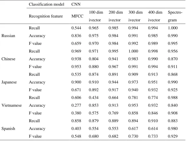
The performance of the six language recognition methods on the five language recognition tasks is shown in Table 1.
Table 1. Summary of the Six Experimental Results
Classification model CNN
Recognition feature MFCC 100 dim
ivector 200 dim ivector 300 dim ivector 400 dim ivector Spectro-gram Russian Recall 0.544 0.965 0.985 0.994 0.994 1.000 Accuracy 0.836 0.975 0.984 0.991 0.985 0.990 F value 0.659 0.970 0.984 0.992 0.989 0.995 Chinese Recall 0.969 0.971 0.995 1.000 0.998 0.956 Accuracy 0.938 0.804 0.941 0.983 0.990 0.870 F value 0.953 0.880 0.967 0.991 0.994 0.911 Japanese Recall 0.535 0.874 0.891 0.909 0.913 0.868 Accuracy 0.900 0.910 0.944 0.973 0.951 0.990 F value 0.671 0.892 0.917 0.940 0.932 0.925 Vietnamese Recall 0.606 0.434 0.664 0.781 0.774 0.988 Accuracy 0.277 0.853 0.913 0.953 0.932 0.840 F value 0.380 0.575 0.769 0.858 0.846 0.908 Spanish Recall 0.858 0.879 0.889 0.894 0.910 0.883 Accuracy 0.403 0.554 0.553 0.617 0.614 0.980 F value 0.548 0.680 0.682 0.730 0.733 0.929
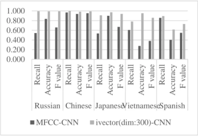
The traditional feature comparison results are shown in Figure 7, the ivector comparison results in different dimensions are shown in Figure 8, and the three feature comparison results are shown in Figure 9.
Figure 7. Comparison of Recognition Results of Traditional Language Recognition Features
Figure 8. Comparison of Ivector Recognition Results in Different Dimensions
Figure 9. Comparison of Language Recognition Feature Recognition Results
0.000 0.200 0.400 0.600 0.800 1.000 Re call Acc ura cy F va lue Re call Acc ura cy F va lue Re call Acc ura cy F va lue Re call Acc ura cy F va lue Re call Acc ura cy F va lue
Russian Chinese JapaneseVietnameseSpanish
MFCC-CNN ivector(dim:300)-CNN 0.000 0.200 0.400 0.600 0.800 1.000
100 dim ivector 200 dim ivector 300 dim ivector 400 dim ivector
0.000 0.100 0.200 0.300 0.400 0.500 0.600 0.700 0.800 0.900 1.000 MFCC Spectrogram ivector
4.4 Result Analysis
From the perspective of the five languages, Russian has the best recognition effect and Vietnamese has the worst recognition. In a sense, it reflects that Russian has more unique pronunciation characteristics than these other four languages, and Vietnamese has the opposite. By comparing traditional language recognition features MFCC and ivector, it is not difficult to find that ivector not only has more free dimensions than MFCC features, it is more convenient to handle, but also better characterizes the language characteristics, which obviously enables better language recognition. It can also be seen from Figure 9 that after the dimensions of the ivector increase to a certain range, the five-language corpus of this experiment cannot continue to improve its recognition effect. Among the four dimensions set, the 300-dimensional ivector achieved the best recognition. Effect, the average F value of the five languages reached 0.902. Finally, in order to verify the recognition effect of the speech recognition method as a feature, a language recognition method based on the sonogram-CNN was set. Because the feature dimension of the speech map is 200 * 400, which is much higher than the ivector dimension, the language it contains It has richer features, but also contains more interference information, but its recognition effect is significantly better than that of ivector on the five-language recognition task. The average F value compares best with the 300-dimensional ivector-CNN recognition method. To improve by 3.5%, up to 0.934.
Generally speaking, the recognition effect is better, referring to previous studies on language recognition (Burget, Matejka, & Cernocky, 2006; Campbell, Richardson, & Reynolds, 2007; Dehak et al., 2009; Dehak et al., 2011; Dehak et al., 2011; Mukherjee et al., 2018; Chaitanya et al., 2018), it is found that the recognition effect is better. The reason may be that the five languages selected in the experiment have large pronunciation differences, which is easier. Identify. Among them, the language recognition method based on the sonogram-CNN can accurately recognize the speech of five languages, probably because the feature data of the sonogram is sufficient, and the author also carried out smaller sonogram features later. Through experiments, it was found that the feature scale of the spectrogram can be reduced within a certain range without affecting the recognition effect, but the order of magnitude is still much larger than the ivector dimension used in the experiment. In general, the number of features is proportional to the computational overhead and to a certain extent proportional to the recognition effect, so the feature recognition of the spectrogram feature is the best, and it is not difficult to find through experiments. The density of language discrimination characteristics is greater, that is, the feature ivector of the same dimension has better recognition effect.
5. Summary
With the emergence of more and more multilingual environments, language recognition technology has become the first link in the process of processing information in various languages, and it has an extremely important role in processing information in various languages. Due to the superposition effect of errors, the accuracy of language recognition directly affects the results of various subsequent
processing processes, so it is necessary to build a language recognition front end with high accuracy and robustness. At present, the development of artificial intelligence is hot, and various deep learning methods are widely used in various subject areas. It has been put into commercial use in the field of image recognition and speech recognition, and has entered people’s daily life. This paper uses experimental methods to compare different language recognition features based on convolutional neural networks, shows the recognition effect of different language recognition features, and analyzes the causes of the recognition results in detail. Based on the comprehensive experimental results, it is the best to use ivector as the language recognition feature for the universal language recognition task. For the five language recognition experiments in this paper, the feature of spectral map feature recognition is the best.
References
Burget, L., Matejka, P., & Cernocky, J. (2006). Discriminative Training Techniques for Acoustic
Language Identification. Acoustics, Speech and Signal Processing, 2006. ICASSP 2006
Proceedings. 2006 IEEE International Conference on 2006.
https://doi.org/10.1109/ICASSP.2006.1659994
Campbell, W. M., Richardson, F., & Reynolds, D. A. (2007). Language Recognition with Word
Lattices and Support Vector Machines. Acoustics, Speech and Signal Processing, 2007.
ICASSP 2007. IEEE International Conference on 2007.
https://doi.org/10.1109/ICASSP.2007.367238
Chaitanya, I. et al. (2018). Word Level Language Identification in Code-Mixed Data using Word
Embedding Methods for Indian Languages. 2018 International Conference on Advances in
Computing, Communications and Informatics (ICACCI), 2018.
https://doi.org/10.1109/ICACCI.2018.8554501
Chen Xin. (2017). On the Interference of Similar Phonemes in Chinese and English to Russian Pronunciation. Overseas English, 20, 221-222.
Dehak, N. et al. (2011) Language Recognition via i-vectors and Dimensionality Reduction.
INTERSPEECH, 2011, 857-860.
Dehak, N. et al. (2011). Front-End Factor Analysis for Speaker Verification. IEEE Transactions on
Audio, Speech and Language Processing, 19(4), 788-798.
https://doi.org/10.1109/TASL.2010.2064307
Dehak, N., Kenny, P., Dehak, R., Glembek, O., Dumouchel, P., Burget, L., … Castaldo, F. (2009).
Support vector machines and Joint Factor Analysis for speaker verification. Acoustics,
Speech and Signal Processing, 2009. ICASSP 2009. IEEE International Conference on 2009. https://doi.org/10.1109/ICASSP.2009.4960564
Han Yi, Wang Guozhen, & Yang Yong. (2008). MFCC-based speech emotion recognition. Journal
597-602.
He Xiangzhi. (2002). Research and Development of Speech Recognition. Computer and
Modernization, 3, 3-6.
Mukherjee, H. et al. (2018). A Dravidian Language Identification System. 2018 24th International
Conference on Pattern Recognition (ICPR), 2018.
https://doi.org/10.1109/ICPR.2018.8545406
Yang Xingjun. (1995). Digital Processing of Speech Signals. Electronics Industry Press.
Yang Xukui, Qu Dan, & Zhang Wenlin. (2014). Orthogonal Laplacian language recognition method. Chinese Journal of Automation, 40(8), 1812-1818.
Yang Xukui. (2015). Information Engineering University, Yang Xukui, etc. Language recognition based on regularized i-Vector algorithm. Journal of Information Engineering University, 16(2), 191-196.
Ye Zinan. (2000). Globalization and Translation of Standardized Languages. China Translators, 02, 8-13.
Yu Jianchao, & Zhang Ruilin. (2009). Speaker recognition based on MFCC and LPCC. Computer
Engineering and Design, 30(05), 1189-1191.
Yu Ming, Yuan Yuqian, Dong Hao, & Wang Zhe. (2006). A text-dependent speaker recognition
method based on MFCC and LPCC. Journal of Computer Applications, 04, 883-885.
Zhang Liyan. (2014). An Analysis of the Transfer of Chinese-English Phonetics to Russian Phonetic Acquisition. Journal of North University of China (Social Science Edition), 30(2), 90-93.
Zhao Fangli. (2012). Russian pronunciation analysis based on praat software. Computer