Bayesian modeling of clustered competing
risks survival times with spatial random
effects
ABSTRACT
In some studies, survival data are arranged spatially such as geographical regions. Incorporating spatial association in these data not only can increase the accuracy and efficiency of the parameter estimation, but it also investigates the spatial patterns of survivorship. In this paper, we considered a Bayesian hierarchical survival model in the setting of competing risks for the spatially clustered HIV/AIDS data. In this model, a Weibull Parametric distribution with the spatial random effects in the form of county-failure type-level was used. A multivariate intrinsic conditional autoregressive (MCAR) distribution was employed to model the areal spatial random effects. Comparison among competing models was performed by the deviance information criterion and log pseudo-marginal likelihood. We illustrated the gains of our model through the simulation studies and application to the HIV/AIDS data.
Key words: Proportional hazards model; Competing risks; Spatial random effect; Markov chain Monte Carlo; HIV; AIDS.
Somayeh Momenyan (1), Amir Kavousi (2), Taban Baghfalaki (3), Jalal Poorolajal (4)
(1)Department of Biostatistics, Shahid Beheshti University of Medical Sciences, Tehran, Iran
(2) Workplace Health Promotion Research Center and Department of Epidemiology, School of Public Health and Safety, Shahid Beheshti University of Medical Sciences, Tehran, Iran
(3) Department of Statistics, School of Mathematical Sciences, Tarbiat Modares University, Tehran, Iran
(4) Research Center for Health Sciences and Department of Epidemiology, School of Public Health, Hamadan University of Medical Sciences, Hamadan, Iran
CORRESPONDING AUTHOR: Amir Kavousi, Department of Biostatistics, Shahid Beheshti University of Medical Sciences, Tehran, Iran. E-mail: kavousi@ sbmu.ac.ir
DOI: 10.2427/13301
INTRODUCTION
In biomedical studies, it is common to have time to event data. In the survival analysis, in many situations, there are some risk factors that are unobservable. In the presence of such risk factors, the usual survival models such as the Cox proportional hazards model are not proper (1). For solving this problem, Vaupel et al. introduced a model with the random effect (2). Clayton and Cuzik introduced the generalization of proportional hazards model by including a random effect to the Cox proportional hazards model to account for variability (3). Frailty models could increase the accuracy and efficiency of the parameter estimation when survival data are independent.
But, in some situations, survival data are dependent such as when a sample of individuals was grouped into clusters. If individuals come from different areas, there will be a spatial correlation between survival data because data from the same or nearer areas are expected to be more similar than those from farther areas (4).
In biostatistics and epidemiology studies, modeling spatial survival data accounting for the spatial association has become popular. For example, Li and Ryan (5) and Banerjee et al. (6) proposed a spatial survival model using the proportional hazards structure from the classical and Bayesian perspective, respectively. The survival model for taking spatiotemporal variation in survival data was investigated by Banerjee and Carlin (6) and Hanson et al. (7). Banerjee and Dey presented semiparametric hierarchical modeling for the proportional odds model in spatially survival data (8). Diva et al. used a Bayesian hierarchical survival model within the proportional hazards and the proportional odds settings (9). Pan et al. proposed a spatial Bayesian semiparametric model to analyze interval-censored survival data (10). More recently, Cramb et al. proposed a spatial flexible
parametric relative survival model (11), and Zhou and Hanson applied the semiparametric survival model with spatial random effects to arbitrarily censored survival data (12).
In the survival data, there is also a situation where, there is more than one cause of failure, but only the occurrence of the first one is observable. (13). The new aspect of this paper is an extension of survival model from single failure type to competing risks in spatially sampled data.
The rest of this paper is outlined as follows. Section 2 describes the HIV/AIDS data. Section 3 formulates our proposed model, including the notations, modeling the cause-specific proportional hazards function with spatial random effects, the prior distribution for areal spatial random effects, and the prior and posterior specification. Section 4 discusses a Bayesian model comparison using deviance information criterion (DIC) (5) and log pseudo-marginal likelihood (LPML) (14). In Section 5, the performance of our model is evaluated through simulation studies. Section 6 analyzes the HIV/AIDS data. Finally, Section 7 presents a discussion of related issues.
THE HIV/AIDS DATA
The data were from a retrospective cohort study, which was conducted in Hamadan Province, the central-western part of Iran, from 1997 to 2011. All 585 HIV-positive people who had a medical record in the HIV testing and treatment centers were included in this study. The explanatory variables included were as follows: age at time of diagnosis, sex, marital status, method of transmission, co-infection with tuberculosis (TB). Also, date of HIV diagnosis, date of progression to AIDS and date of death (if any) and patient’s county of residence were collected. The main outcome in this study was the time
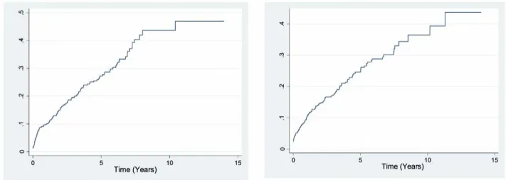
interval, between HIV diagnosis and AIDS progression, so the event of interest was AIDS progression. However, some of HIV infected patients die before AIDS progression. Thus, death before AIDS was considered as competing risk. The patients who did not experience any of these events or were lost to follow-up were considered as censored. Accordingly, in the final outcome classification, patients were categorized into three categories: those who developed AIDS (23.4%), those who died post-HIV infection (22.9%), and those who censored (53.7%). Figure 1 plotted the observed cumulative incidence curve for risks of AIDS progression and mortality post-HIV infection. As seen, the cumulative incidence probability for AIDS progression is higher than competing event of death after the first 5 years.
MODEL FORMULATION
In this section, we suppose n individuals come from K counties. nkis the number of individuals in a sample in
each county, where k = 1,..., K and ΣK
k=1 nk = n. Also, let
Cik = (Tik,δik) be the data for the i-th individual living in the
k-th county, i = 1,..., nk, where Tik denotes time to an event
which may be right censored time. In competing risks data, each individual has one of the G possible failure types during follow-up or could be right censored. Hence, failure type indicator or δik takes value from {0,1,...,G}.
Survival model with random effects
Different models for analyzing competing risks data have been proposed in the last three decades (15, 16). The typical approach for analyzing competing risks survival times is modeling the cause-specific hazard functions (17).
where h0(t)g is an unspecified baseline risk function and
βg = (βg
1,β2g,...,βpg) is a p x 1 vector of regression parameters
associated to a p x 1 vector of observed explanatory covariates xik = (xik1, xik2,..., xikp) for the gth type of failure
where g = 1,..., G. In this model, to estimate the hazard of each failure type, other competing risks are assumed as censored in addition to those who are censored from loss to follow-up. But, sometimes, those who experience competing risk events are censored informatively; because of that, in the competing risks setting, the assumption of independent censoring is no longer reasonable. For example, in the HIV/AIDS data, the factors that affect the risk of AIDS progression as the event of interest might also influence the probability of mortality post-HIV infection as the competing risk event. To avoid biased results, we introduce the random effects V = (V1,...,VG)T, to capture
for the association between times of different failure types; for more details, see Huang and Wolfe (18) and also Christian et al. (19). We introduce these random effects through (1), as
hg
ik (t|xik,vgik) = h0(t)g exp (xTikβg + vikg) (2)
On the other hand, since subjects come from different counties, we consider a survival model with the spatial random effects. Let Wg
k, k = 1,...,K, g=1,..., G, denotes the
spatial random effects. We introduce again, these random effects through (2), as
hg
ik (t|xik,vgik, Wgk) = h0(t)g exp (xTikβg + vik g+ Wgk) (3)
Alternatively, for the baseline hazard function, we assume a cause-specific Weibull function, which is
h0(t)g = pgt pg-1 with the shape parameter pg for the g-th type
of failure. Hence, the model (3) can be substituted by:
hg
ik (t|xik,Vikg, Wgk) = pgt pg-1 exp (xTikβg + Vgik + Wkg) (4)
Spatial random effects
A common model for areal data collected over a geographic region in a univariate case such as a single disease is the conditional autoregressive (CAR) distribution, developed by Besage (20). Let W = (W1,...,WK)T be the spatial
random effects vector observed at the K areal counties, then the general form of the CAR joint distribution is
W ~ N (0, [σ2
w D (I - αB)]-1) (5)
where B is a K x K matrix, ο2
w is conditional variance
and α is called a smoothing parameter. If we specify D = diag (mk), mk is the number of neighbors of the k-th
county, and B = D-1 B
w where Bw is the adjacency matrix
of the graph representing our county (bw k k = 0, bw k k = 1 if the county k is a neighbor of the county k, bw k k if the county k is not a neighbor of the county k), we obtain the so-called intrinsic conditional autoregressive (ICAR) distribution that is the most common CAR distribution (21). Also, in this structure, we set the smoothing parameter α = 1. This distribution is denoted as CAR (1, σ2
w ) and its
formulation, thus becomes
W ~ N (0, σ22
w Σ-1w), (6)
where Σw = (D - Bw) is a K x K matrix. But, when we
have the multivariate areal data, such as information on multiple diseases over the same regions, the multivariate areal models are proper for analyzing this kind of data (22, 23). There are several multivariate areal models that have been proposed in the literature. The multivariate Normal Markov random field (MRF) was proposed by hg
ik (t|xik) = lim
p (t≤Tik<t+dt,δik=g|Tik≥t,xik)
dt
dt → 0 = h0 (t)
gexp(xT ikβg),
Mardia (24). A twofold CAR model for two diseases and multi-objective version of the CAR model were proposed by Kim et al. (25) and sain and Cressie (26), respectively. The multivariate CAR models for the hierarchical modeling based on MRF have been proposed by Carlin and Banerjee (27) and Gelfand and Vounatsou (28). In this paper, we use the multivariate intrinsic conditionally autoregressive (MCAR) distribution for the spatial random effects in the HIV/AIDS data to be able to model the possible correlation in the risks of AIDS progression and mortality post-HIV infection over the same counties as well as the possible spatial correlation among the counties. Let W = (WT
1,...,WTK)T where W is KG x 1 with each Wk =
(W1
k ,...,WGk)T being a G-dimensional vector of the spatial
random effects collection for the G possible failure types within the k-th county. The joint distribution for W takes the following form
W ~ N (0 [D (I - αB), ⊗ Λ]-1). (7)
If we postulate D, B, and α similar to ICAR distribution that was mentioned above, we obtain the multivariate intrinsic conditional autoregressive distribution. This distribution is denoted as MCAR (1,Λ) and its formulation is also equivalent to
W ~ N (0, (Σw⊗ Λ)-1), (8)
where Σw = (D - Bw) is a K x K matrix and therefor
Σw ⊗ Λ is a KG x KG matrix. Moreover, Λ is a G x G
positive definite and symmetric matrix, which is defined as the variance-covariance matrix of the spatial failure type and controls the correlation between the competing risks in the survival process at any given county. Note that, in this setup, we are modeling the dispersion matrix of the spatial-by-failure type interaction, W, as the Kronecker product of the spatial dispersion and the failure type dispersion. Also, we use the same Λ for all of the counties.
Likelihood
Let θ = (βg,Λ, Wg
k, vikg, p ; i = 1,..., ng k, k=1,...K, g=1,...G)
denotes all the unknown parameters and
(Cik, Xik; i=1,..., nk, k=1,..., K) represents the observed data;
therefore, the likelihood function for this model is product of all n individual contributions to the likelihood
L (θ| C,X) α
∏ ∏
Lik (θ| Cik,xik) (9)Considering the distribution of competing risks survival response, Lik (θ| Cik,xik) is as follows:
∏
[
[pgt pg-1 exp (xTikβg + vik g+ Wgk)]I(δik=g) (10)
x exp
[
-∫
0 pgt pg-1 exp (xTikβg + Vik g+ Wgk)dt]]
Finally, the likelihood for θ, conditional on the observed data is expressed as follows,
∏ ∏
[
∏
[
pgt pg-1 [exp(xTikβg + Vik g+ Wgk)]I(δik=g) (11)
x exp
[
-∫
0 pgt pg-1 exp (xTikβg + Vgik + Wgk)d]]
]
Bayesian approach
In the Bayesian approach, we considered the prior distribution for all parameters. The standard non-informative prior distributions for the parameters were considered as follows: for the regression coefficients,βg, and the Weibull
shape parameters, pg; g = 1,...; G; a multivariate Normal,
N (0, Σβ), and a gamma, G (a1, b1), priors were taken
respectively. We assumed for vg
ik; i = 1,...,nk,k = 1,..., K, g = 1,...,G a multivariate Normal
distribution, that is Vik~N (0,Λ) where Λ is a G x G
variance-covariance matrix. Concerning the spatial random effects, we used the MCAR prior distribution, W ~ MCAR (1,Λ), (see section 3.2). For the variance-covariance matrix, Λ an inverse Wishart, JW (R, v), was used where matrix R is a G x G positive definite matrix and v is degrees of freedom. Thus, in our model, we are using the same Λ to model the MCAR and failure type random effects distributions. For all these priors, we chose the distributions with the very high variance. The joint posterior distribution of our proposed model is denoted by π (θ|C,X), and is proportional to
L (θ|C,X)x π (βg|Σ
β) x π (pg| a1,b1) x π (V,Λ) x π (W|Σw,Λ) x π (Λ|R,v).
(12)
After initializing values for the parameters, sampling from the full conditional distribution by the MCMC algorithm was performed. All statistical analysis and also mapping the results were performed using OpenBUGS software (29), version 3.2.3, GeoBUGS and R package R2OpenBUGS (30, 31).
MODEL SELECTION
We selected two summary measures for the model selection as follows: the deviance information criterion (DIC) and log pseudo-marginal likelihood (LPML). The DIC criterion for model m is defined as follows:
nk
i=1 k=1
K
G
g=1 t
ik
tik K nk G
DIC (m) = -2D[θm ,m] - D [θm ,m] = D [θm ,m] + 2pm,
(13)
where D[θm ,m] is the deviance measure and is defined as: D[θm ,m] = -2log f (Y|θm ,m),
and D[θm ,m] is its posterior mean. Also, θm is the posterior mean of the parameters involved in model m and pm is an
effective number of parameters of model m and is defined as follows:
pm= D[θm ,m] - D [θm ,m].
The model with the smallest of DIC is the preferred model between a collection of alternative models. LPML statistic is based on the conditional predictive ordinate (CPO). The CPO statistic for ikth individual is defined as predictive density based on all of data except ikth individual. The high value of CPO statistic indicates that data for subject can be truly predicted by a model based on data from all other subjects. The LPML is used as an overall measure of the model fit and is calculated as:
LPML =
Σ
log (CPOik). (14)A model with a maximum value of LPML implies a better model. Using the MCMC methods, the DIC and LPML compute from the posterior samples.
SIMULATION STUDY
The performance of our model was evaluated through a series of scenarios in the simulation study. We generated a total of 100 simulated datasets with three levels of sample size in each county (nk=50, nk =100, nk =200)
and with three censoring rate (low, 20%, medium, 40%, and high, 60%). For each dataset, the neighborhood structure was based on the nine counties in Hamadan, Iran. We used a continuous covariate (X1) and a binary
categorical covariate (X2) that was generated from a
standard Normal distribution and a Bernoulli distribution with a success probability p = 0.5, respectively. Also, we simulated two competing risks, risk 1 and 2, from the cause-specific exponential model. The failure times were generated based on the algorithm that Beyersmann and et al. presented for Competing risks data (32). As for each individual, the event time was generated by overall hazard rate that at each time point was the sum of cause-specific hazard rates for two types of event, λik(t) = λ1ik(t) + λ2ik(t).
The cause-specific hazard rate for each type of event was considered as follows in each county
λ1
ik(t|xik,V1ik) = exp (β11x1ik +β12x2ik +V1ik +W1k),
λ2
ik(t|xik,V2ik) = exp (β21x1ik +β22x2ik +V2ik +W2k).
The type of event was determined by a Bernoulli experiment with the probability P1= λ1 λ for the event of type 1 and
P2= λ2 λ for the event of type 2. The random effects Vik,
were generated from a multivariate Normal with a mean 0 and a 2 x 2 covariance matrix of Λ, that Λ11= 0.1, Λ22= 0.1 and Λ12= 0.05 and then were centered around its mean. Also, the spatial random effects W,were generated from the MCAR distribution, N (0, (Σ*-1
w⊗Λ)) where Σ*w=0.99xΣw
+ diag (0.01), and then were centered around its mean. We introduced Σ*
w to be invertible the precision matrix
and centered to be identifiable the spatial random effects. The corresponding regression coefficients were set β1
1=0.6,
β1
2=-0.4. for risk 1 and β21=-0.3, β22=0.7 for risk 2. The matrix
R was set as 0.1I2x2. The data above a threshold were right
censored which were selected as the (1-α) -quantile of the sample survival times, such that 100α% of the observations were censored.
For each of the fitted models, the convergence of the MCMC chain was evaluated by trace plot, auto-correlation plot, and Gelman-Rubin’s diagnostic (33). For each MCMC chain, we run the 25,000 iterations. For each parameter, the point estimate, bias, and mean square error (MSE) were calculated by the average of the means, biases and the square errors from the 100 replicates, respectively. The coverage probability (CP) was calculated as the proportion of the 95% credible intervals that contain the true values. The bias and square error are defined as:
Bias (θ) = (θi-θ), SE(θ) = (θi-θ)2.
Simulation results
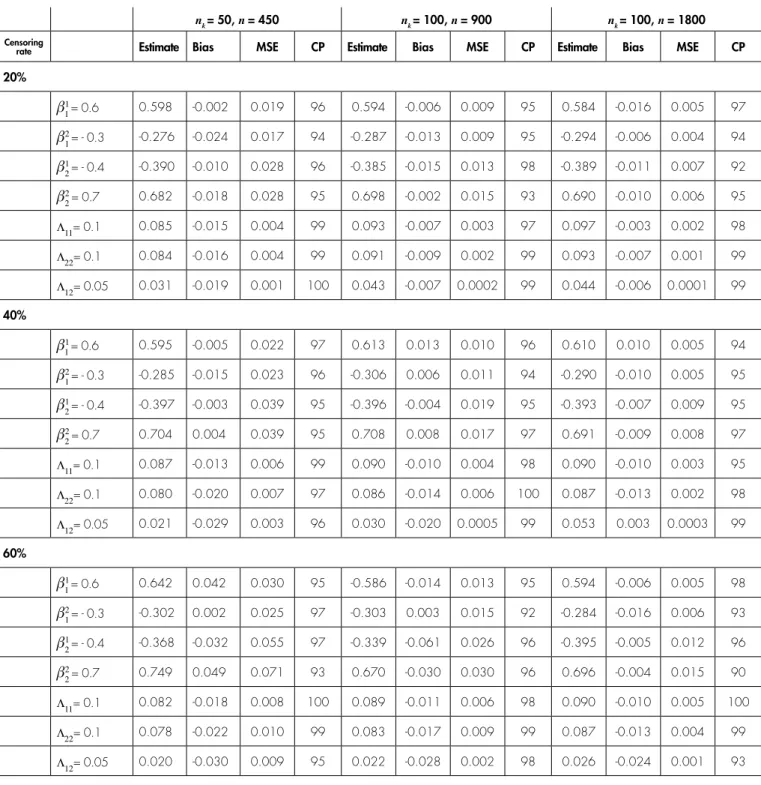
The results of the simulation study from nine scenarios are reported in Table 1. While estimation of the regression coefficients in the total scenario were close to the truth value 1, but estimation of the covariance matrix Λ had a consistently small bias for the large sample size (nk = 200)
and with censoring rate 20% and 40%. Also, all parameters had the coverage probabilities close to the nominal level of 0.95 under all the scenarios. The MSE criterion for all parameters was close together and as sample size increases, the estimation accuracy of parameters increases.
ANALYSIS OF THE HIV/AIDS DATA
We analyzed the HIV/AIDS data using four models as follows:
Model 1: The model with any random effects in the log-relative hazard (xTβg ),
nk = 50, n = 450 nk = 100, n = 900 nk = 100, n = 1800
Censoring
rate Estimate Bias MSE CP Estimate Bias MSE CP Estimate Bias MSE CP
20%
β1
1 = 0.6 0.598 -0.002 0.019 96 0.594 -0.006 0.009 95 0.584 -0.016 0.005 97
β2
1 = - 0.3 -0.276 -0.024 0.017 94 -0.287 -0.013 0.009 95 -0.294 -0.006 0.004 94
β1
2 = - 0.4 -0.390 -0.010 0.028 96 -0.385 -0.015 0.013 98 -0.389 -0.011 0.007 92
β2
2 = 0.7 0.682 -0.018 0.028 95 0.698 -0.002 0.015 93 0.690 -0.010 0.006 95 Λ11= 0.1 0.085 -0.015 0.004 99 0.093 -0.007 0.003 97 0.097 -0.003 0.002 98
Λ22= 0.1 0.084 -0.016 0.004 99 0.091 -0.009 0.002 99 0.093 -0.007 0.001 99
Λ12= 0.05 0.031 -0.019 0.001 100 0.043 -0.007 0.0002 99 0.044 -0.006 0.0001 99
40%
β1
1 = 0.6 0.595 -0.005 0.022 97 0.613 0.013 0.010 96 0.610 0.010 0.005 94
β2
1 = - 0.3 -0.285 -0.015 0.023 96 -0.306 0.006 0.011 94 -0.290 -0.010 0.005 95
β1
2 = - 0.4 -0.397 -0.003 0.039 95 -0.396 -0.004 0.019 95 -0.393 -0.007 0.009 95
β2
2 = 0.7 0.704 0.004 0.039 95 0.708 0.008 0.017 97 0.691 -0.009 0.008 97 Λ11= 0.1 0.087 -0.013 0.006 99 0.090 -0.010 0.004 98 0.090 -0.010 0.003 95
Λ22= 0.1 0.080 -0.020 0.007 97 0.086 -0.014 0.006 100 0.087 -0.013 0.002 98
Λ12= 0.05 0.021 -0.029 0.003 96 0.030 -0.020 0.0005 99 0.053 0.003 0.0003 99
60%
β1
1 = 0.6 0.642 0.042 0.030 95 -0.586 -0.014 0.013 95 0.594 -0.006 0.005 98
β2
1 = - 0.3 -0.302 0.002 0.025 97 -0.303 0.003 0.015 92 -0.284 -0.016 0.006 93
β1
2 = - 0.4 -0.368 -0.032 0.055 97 -0.339 -0.061 0.026 96 -0.395 -0.005 0.012 96
β2
2 = 0.7 0.749 0.049 0.071 93 0.670 -0.030 0.030 96 0.696 -0.004 0.015 90 Λ11= 0.1 0.082 -0.018 0.008 100 0.089 -0.011 0.006 98 0.090 -0.010 0.005 100
Λ22= 0.1 0.078 -0.022 0.010 99 0.083 -0.017 0.009 99 0.087 -0.013 0.004 99
Λ12= 0.05 0.020 -0.030 0.009 95 0.022 -0.028 0.002 98 0.026 -0.024 0.001 93
TABLE 1. Estimation results for the simulation study
Log-relative hazard LPML DIC (Model 1) xT
ik βg -963.11 1908.00
(Model 2) xT
ik βg + Wk -962.60 1906.00
(Model 3) xT
ik βg + Vikg + Wgk -962.76 1906.00
(Model 4) xT
ik βg + Vikg + Wgk -958.78 1903.00
(xT
ik βg + Wk; W ~ N (0, Σ-1w)),
Model 3: The model with the spatial and non-spatial failure type random effects in the log-relative hazard
(xT
ik βg + Vikg + Wgk; W ~ N (0,I Σ-1KxK⊗Λ)),
Model 4: The model with the multivariate spatial and failure type random effects in the log-relative hazard
(xT
ik βg + Vikg + Wgk; W ~ N (0,I Σ-1w⊗Λ)).
The first model is the model that does not account for the correlation between the competing risks in the survival process and also the spatial correlation among the counties. The second model is the model that only incorporates the spatial variation among the counties. In this model, we considered the ICAR prior distribution for the univariate spatial random effects (see section 3.2) and also for the spatial random effects variance σ22
w an inverse-gamma, IG
(a2,b2) prior was used. The third model is the spatially
independent model with basically the same structure with our proposed model. The spatially independent model was accomplished by replacing the Σwwith a diagonal
matrix which does not account for the spatial structure of the counties, whence the collection of independent random effects for G failure types within the county, denoted by W has a N (0,(I-1
KxK⊗Λ)) distribution. In other words, in this
model, we consider the spatial and non-spatial failure type random effects in the log-relative hazard. The fourth model is the full model that we proposed in this paper.
The proposed models were fitted based on sampling chains of 100,000 iterations with a spacing of 10 for reducing level of correlation and the first 10,000 discarded as a burn-in. Trace, auto-correlation and density plots of the posterior distributions were assessed for convergence of the MCMC chains. The Gelman-Rubin’s statistics for all parameters were between 1.0 and 1.1. The consistent batch means estimates of Monte Carlo standard errors were from 0.00002 to 0.0002 for all parameters. The summary measures of all parameters consist of the mean and standard deviation by posterior samples were obtained. Moreover, for the regression coefficients, the adjusted hazard ratios (HR) were calculated with 95% credible intervals.
Table 2 compared four models based on two criteria, DIC and LPML. The DIC and LPML values for the four proposed models were very close, but model 4 which introducing the multivariate spatial and failure type random effects, showed somewhat better comparison measure values. In addition, these values suggested that each of these models is better than the first model that does not account for any correlation. The summary measures of all parameters of the fourth model were presented in Table 3. Also, because the MCAR distribution is improper and parameterized to include a sum-to-zero constraint on the
random effects, a separate intercept coefficient for each of two risks with a flat prior was included in this model.
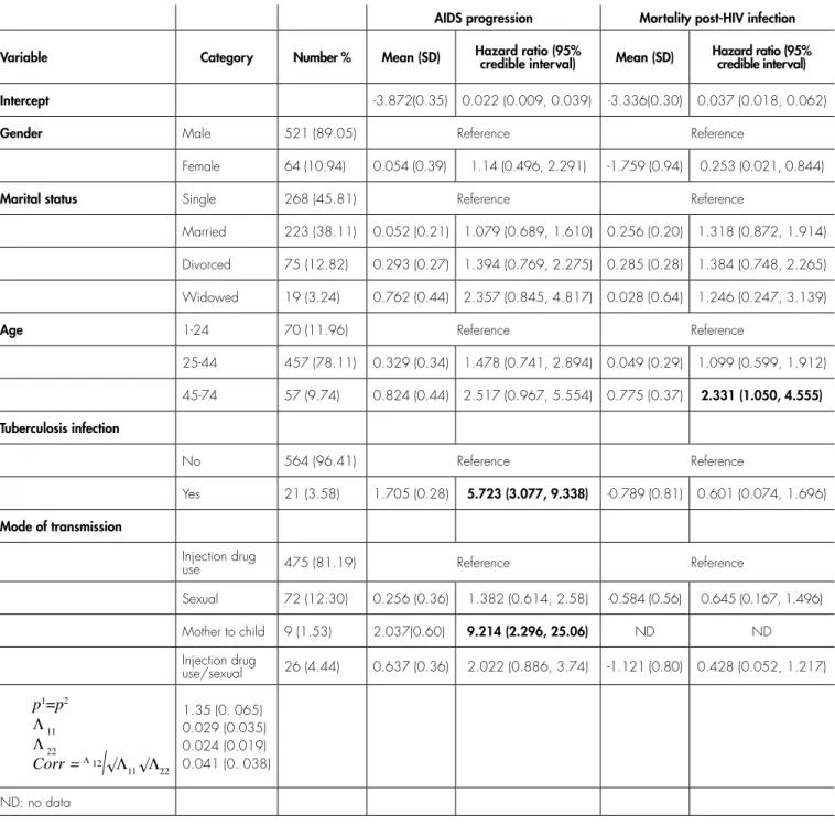
Based on the adjusted HR estimates, there were the significant relationships between TB co-infection and mode of transmission with the risk of AIDS progression. However, the adjusted relationships for the risk of mortality post-HIV infection were not statistically significant for all the predictors except age at diagnosis. In other words, HIV-positive patients who were co-infected with TB and became infected through mother to child had a higher risk of AIDS progression as compared to those who were infected with HIV alone and infected through IDU. Also, the risk of mortality post-HIV infection was higher in patients aged 45 to 74 years than in those aged 0 to 24 years, such that the adjusted HR was 2.33.
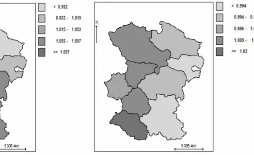
We also mapped the summaries of our results. Figure 2 shows 2 maps that represent the posterior spatial relative risk in nine counties of Hamadan Province. The map on the left is for the relative risk of AIDS progression and the map on the right is for the relative risk of mortality post-HIV infection that is defined by exp (W1
w) and exp (W2w)
respectively. The posterior estimates of county-specific random effects were recorded based on the quintile of their distribution for showing the spatial inequalities on the map. As shown in Figure 2, for the risk of AIDS progression, one cluster of counties was identified with higher risk in the south, southeast, and southwest regions (six out of nine counties) and one cluster with lower risk in the north, northeast, and northwest regions (three out of nine counties) was identified. Also, for the risk of mortality post-HIV infection, the high-risk cluster consists of the northwest, west, and southwest regions (five out of nine counties) and the low-risk cluster consists of the northeast, east, and southeast regions (four out of nine counties). The posterior correlation between risks of AIDS progression and mortality post-HIV infection was shown in Table 3. The coefficient of correlation was 0.04 suggesting a weak shared geographical and overall pattern between the risks of AIDS progression and mortality post-HIV infection. Finally, with regard to modeling details, using a vague inverse Wishart, IW (R,v) for Λ where v=7 and R=0.1I2x2
leads to acceptable convergence behavior.
DISCUSSION
was good in terms of efficiency and accuracy of parameters estimation. As far as we know, our proposed model is new in survival data and could help in the visual representation of the spatial relative risk inequalities for each risk. This information also could be valuable for public health institutes and health researchers. In other words, despite the fact that we had a limited gain we analyzed the HIV/ AIDS data using model 4 for its interesting clinical results. Hence, introducing this model in our dataset could be useful in similar datasets in clinical research in the future. In other words, clinical researches in the area of HIV/AIDS
can produce interesting clinical results using model 4. According to the posterior estimates of adjusted HR, there were the significant associations between TB co-infection and mode of transmission with risk of AIDS progression. Also, there was the significant association between age at diagnosis with risk of mortality post-HIV infection. It should be mentioned that the estimated regression coefficients of cause-specific proportional hazards model give the effect of covariates on the instantaneous hazard for the type of failures and cannot be interpreted to an effect on the cumulative
AIDS progression Mortality post-HIV infection Variable Category Number % Mean (SD) Hazard ratio (95% credible interval) Mean (SD) Hazard ratio (95% credible interval) Intercept -3.872(0.35) 0.022 (0.009, 0.039) -3.336(0.30) 0.037 (0.018, 0.062)
Gender Male 521 (89.05) Reference Reference
Female 64 (10.94) 0.054 (0.39) 1.14 (0.496, 2.291) -1.759 (0.94) 0.253 (0.021, 0.844)
Marital status Single 268 (45.81) Reference Reference
Married 223 (38.11) 0.052 (0.21) 1.079 (0.689, 1.610) 0.256 (0.20) 1.318 (0.872, 1.914) Divorced 75 (12.82) 0.293 (0.27) 1.394 (0.769, 2.275) 0.285 (0.28) 1.384 (0.748, 2.265) Widowed 19 (3.24) 0.762 (0.44) 2.357 (0.845, 4.817) 0.028 (0.64) 1.246 (0.247, 3.139)
Age 1-24 70 (11.96) Reference Reference
25-44 457 (78.11) 0.329 (0.34) 1.478 (0.741, 2.894) 0.049 (0.29) 1.099 (0.599, 1.912) 45-74 57 (9.74) 0.824 (0.44) 2.517 (0.967, 5.554) 0.775 (0.37) 2.331 (1.050, 4.555) Tuberculosis infection
No 564 (96.41) Reference Reference
Yes 21 (3.58) 1.705 (0.28) 5.723 (3.077, 9.338) -0.789 (0.81) 0.601 (0.074, 1.696)
Mode of transmission
Injection drug
use 475 (81.19) Reference Reference
Sexual 72 (12.30) 0.256 (0.36) 1.382 (0.614, 2.58) -0.584 (0.56) 0.645 (0.167, 1.496) Mother to child 9 (1.53) 2.037(0.60) 9.214 (2.296, 25.06) ND ND Injection drug
use/sexual 26 (4.44) 0.637 (0.36) 2.022 (0.886, 3.74) -1.121 (0.80) 0.428 (0.052, 1.217)
p1 =p2 Λ 11 Λ 22
Corr =Λ 12
�Λ11 �Λ22
1.35 (0. 065) 0.029 (0.035) 0.024 (0.019) 0.041 (0. 038) ND: no data
incidence function. In other words, in the cause-specific hazard model, the effect of same covariates is modeled for competing events, so there is no direct connection between the regression coefficients and the cumulative incidence functions. The reason is that the cumulative incidence function for the type of failure depends not only on the hazard of the type of failure, but also on the hazards of all other failure types. Thus, the relation of one covariate with the cumulative incidence functions of the type of failure depends on the effects of a covariate on all failure types (13, 17).
In the field of HIV/AIDS disease, understanding of geographic variation of risks of AIDS progression and mortality post-HIV infection provides greater opportunity to identify high-burden areas, since they reflect both diagnostic and patient management. From the results of present study, the low-risk cluster in risk of AIDS progression contained counties with lowest population density and the high-risk cluster in risk of AIDS progression consists of some counties with the highest rate of population density. Also, the low-risk cluster was in remote areas and with much distance from the most populous counties in Hamadan Province. In order to take more spatial variation in the HIV/ AIDS data, instead of counties another smaller regions should be used, that unfortunately, were not available in our data.
Our results showed a small positive correlation between hazards of AIDS progression and mortality post-HIV infection that this information is not available when each failure type is modeled independently. We used the same variance-covariance matrix to model the MCAR and failure type random effects distributions as mentioned
before, but we could not generalize in a way that the model accounts for the different spatial and non-spatial failure type variance-covariance matrices because of the identifiability problem.
Acknowledgments
Receiving support from the Center of Excellence in Analysis of Spatio-Temporal Correlated Data at Tarbiat Modares University is acknowledge.
Declaration of conflicting interests
No conflict of interest has been declared by the authors with respect to the research, authorship, and/or publication of this paper.
Funding
There is no financial support for this research.
References
1. Motarjem K, Mohammadzadeh M, Abyar A. Geostatistical survival model with Gaussian random effect. Statistical Papers. 2017:1-23. 2. Vaupel JW, Manton KG, Stallard E. The impact of heterogeneity
in individual frailty on the dynamics of mortality. Demography. 1979;16(3):439-54.
3. Clayton D, Cuzick J. Multivariate generalizations of the proportional hazards model. Journal of the Royal Statistical Society Series A (General). 1985:82-117.
4. Banerjee S, Carlin BP, Gelfand AE. Hierarchical modeling and analysis for spatial data: CRC press; 2014.
5. Spiegelhalter DJ, Best NG, Carlin BP, Van Der Linde A. Bayesian measures of model complexity and fit. Journal of the Royal Statistical Society: Series B (Statistical Methodology). 2002;64(4):583-639. 6. Banerjee S, Wall MM, Carlin BP. Frailty modeling for spatially
correlated survival data, with application to infant mortality in Minnesota. Biostatistics. 2003;4(1):123-42.
7. Hanson TE, Jara A, Zhao L. A Bayesian semiparametric temporally-stratified proportional hazards model with spatial frailties. Bayesian Analysis. 2012;7(1):147-88.
8. Banerjee S, Dey DK. Semiparametric proportional odds models for spatially correlated survival data. Lifetime data analysis. 2005;11(2):175-91.
9. Diva U, Dey DK, Banerjee S. Parametric models for spatially correlated survival data for individuals with multiple cancers. Statistics in medicine. 2008;27(12):2127-44.
10. Pan C, Cai B, Wang L, Lin X. Bayesian semiparametric model for spatially correlated interval-censored survival data. Computational Statistics & Data Analysis. 2014;74:198-208.
11. Cramb SM, Mengersen KL, Lambert PC, Ryan LM, Baade PD. A flexible parametric approach to examining spatial variation in relative survival. Statistics in medicine. 2016;35(29):5448-63. 12. Zhou H, Hanson T. A Unified Framework for Fitting Bayesian
Semiparametric Models to Arbitrarily Censored Survival Data, Including Spatially Referenced Data. Journal of the American Statistical Association. 2018;113(522):571-81.
13. Putter H, Fiocco M, Geskus RB. Tutorial in biostatistics: competing risks and multi-state models. Statistics in medicine. 2007;26(11):2389-430.
14. Gelfand AE, Dey DK, Chang H. Model determination using predictive distributions with implementation via sampling-based methods. STANFORD UNIV CA DEPT OF STATISTICS; 1992. 15. Haller B, Schmidt G, Ulm K. Applying competing risks regression
models: an overview. Lifetime data analysis. 2013;19(1):33-58. 16. Pintilie M. Competing risks: a practical perspective: John Wiley &
Sons; 2006.
17. Fine JP, Gray RJ. A proportional hazards model for the subdistribution of a competing risk. Journal of the American statistical association. 1999;94(446):496-509.
18. Huang X, Wolfe RA. A frailty model for informative censoring.
Biometrics. 2002;58(3):510-20.
19. Christian NJ, Ha ID, Jeong JH. Hierarchical likelihood inference on clustered competing risks data. Statistics in medicine. 2016;35(2):251-67.
20. Besag J. Spatial interaction and the statistical analysis of lattice systems. Journal of the Royal Statistical Society Series B (Methodological). 1974:192-236.
21. Besag J, Kooperberg C. On conditional and intrinsic autoregressions. Biometrika. 1995;82(4):733-46.
22. Torabi M. Spatial generalized linear mixed models with multivariate CAR models for areal data. Spatial Statistics. 2014;10:12-26. 23. Jin X, Carlin BP, Banerjee S. Generalized hierarchical multivariate
CAR models for areal data. Biometrics. 2005;61(4):950-61. 24. Mardia K. Multi-dimensional multivariate Gaussian Markov random
fields with application to image processing. Journal of Multivariate Analysis. 1988;24(2):265-84.
25. Kim H, Sun D, Tsutakawa RK. A bivariate Bayes method for improving the estimates of mortality rates with a twofold conditional autoregressive model. Journal of the American Statistical Association. 2001;96(456):1506-21.
26. Sain SR, Cressie N. Multivariate lattice models for spatial environmental data. Proc Statist Environ Sect Am Statist Ass. 2002:2820-5.
27. Carlin B, Banerjee S, editors. Hierarchical Multivariate CAR Models for Spatio-Tempo rally Correlated Survival Data. Bayesian Statistics 7: Proceedings of the Seventh Valencia International Meeting; 2003: Oxford University Press, USA.
28. Gelfand AE, Vounatsou P. Proper multivariate conditional autoregressive models for spatial data analysis. Biostatistics. 2003;4(1):11-5.
29. Lunn D, Spiegelhalter D, Thomas A, Best N. The BUGS project: Evolution, critique and future directions. Statistics in medicine. 2009;28(25):3049-67.
30. Sturtz S, Ligges U, Gelman A. R2OpenBUGS: a package for running OpenBUGS from R. URL http://cran rproject org/web/ packages/R2OpenBUGS/vignettes/R2OpenBUGS pdf. 2010. 31. Team RC. R: A language and environment for statistical computing.
BM Corporation, Armonk, NY. R version 3.0. 1 R Foundation for Statistical Computing, Vienna, Austria. 2015.
32. Beyersmann J, Latouche A, Buchholz A, Schumacher M. Simulating competing risks data in survival analysis. Statistics in medicine. 2009;28(6):956-71.