Cometary compositions compared with protoplanetary disk midplane chemical evolution. An emerging chemical evolution taxonomy for comets

(1)

July 29, 2019

Cometary compositions compared with protoplanetary disk

midplane chemical evolution

An emerging chemical evolution taxonomy for comets

Christian Eistrup

1,2,?

, Catherine Walsh

3

and Ewine F. van Dishoeck

1,4

1 _{Leiden Observatory, Leiden University, P. O. Box 9531, 2300 RA Leiden, The Netherlands}

2 _{Department of Astronomy, University of Virginia, 530 McCormick Road, 22903 Charlottesville, VA, USA}

e-mail:[email protected]

3 _{School of Physics and Astronomy, University of Leeds, Leeds, LS2 9JT, UK}

4 _{Max-Planck-Institut für Extraterrestriche Physik, Giessenbackstrasse 1, 85748 Garching, Germany}

Received· · ·/Accepted· · ·

ABSTRACT

Context.Comets are planetesimals left over from the formation of planets in the solar system. With a growing number of observed molecular abundances in many comets, and an improved understanding of chemical evolution in protoplanetary disk midplanes, comparisons can be made between models and observations that could potentially constrain the formation histories of comets.

Aims.Our aim is to carry out the first statistical comparison between cometary volatile ice abundances and modelled evolving abun-dances in a protoplanetary disk midplane.

Methods.Aχ2_{-method was used to determine maximum likelihood surfaces for 14 di}_ff_{erent comets that formed at a given time (up to}

8 Myr) and place (out to beyond the CO iceline) in the pre-solar nebula midplane. This was done using observed volatile abundances for the 14 comets and the evolution of volatile abundances from chemical modelling of disk midplanes. Two assumptions for the chemical modelling starting conditions (cloud inheritance or chemical reset), as well as two different sets of cometary molecules (parent species, with or without sulphur species) were investigated.

Results.Considering all parent species (ten molecules) in the reset scenario,χ2_{likelihood surfaces show a characteristic trail in the}

parameter space with high likelihood of formation around 30 AU at early times and 12 AU at later times for ten comets. This trail roughly traces the vicinity of the CO iceline in time.

Conclusions.A statistical comparison between observed and modelled chemical abundances in comets and comet-forming regions could be a powerful tool for constraining cometary formation histories. The formation histories for all comets were constrained to the vicinity of the CO iceline, assuming that the chemistry was partially reset early in the pre-solar nebula. This is found, both when considering carbon-, oxygen-, and sulphur-bearing molecules (ten in total), and when only considering carbon- and oxygen-bearing molecules (seven in total). Since these 14 comets did not previously fall into the same taxonomical categories together, this chemical constraint may be proposed as an alternative taxonomy for comets. Based on the most likely time for each of these comets to have formed during the disk chemical evolution, a formation time classification for the 14 comets is suggested.

Key words. astrochemistry – protoplanetary disks – comets: general

1. Introduction

When the solar system formed 4.6 billion years ago, the planets formed their cores from solid material in the pre-solar nebula. In the outer, colder regions of this nebula volatile molecules, such as H₂O, CO₂, and CO were frozen out as ices on the surfaces of grains, and later larger bodies. Some of these bodies merged to form the planetary cores, and eventually the Jovian planets, but some of this solid material remained unused by planets and is still present as comets in our solar system today .

Comets are made up of partly refractory dust and partly volatile ices. These ices reside deep inside the comets, and they are thought to be pristine samples of the material that was present in the pre-solar nebula (see review by Mumma & Charnley 2011). Comets are thus interesting because of what they can tell us about the chemical composition in the icy outer pre-solar neb-ula 4.6 billion years ago, but also because comets are known to

? _{Virginia Initiative on Cosmic Origins (VICO) Fellow}

have impacted on the Earth after having been dynamically scat-tered towards the Sun from the outer solar system. The volatile and organic material they carry on them has thus added to the chemical make-up of the Earth. Furthermore, understanding the origin of water and life on Earth may be traced back to comets.

Comets have been observed from the ground and from space for decades in various wavelength regimes (see e.g. Biver et al. 1999, 2014; Bockelée-Morvan et al. 2000, 2015). Several ef-forts have gone into detecting molecular species in the comae of comets and using these to classify them (A’Hearn et al. 1995; Fink 2009; Mumma & Charnley 2011; Cochran et al. 2012; Le Roy et al. 2015). At least two classification groups have been proposed for cometary compositions: ‘typical’ and ‘depleted’, where depleted refers to a depletion in organic carbon-chain molecules, compared with the typical compositions (see e.g. Cochran et al. 2012). Hundreds of comets have been analysed for composition. The majority of these (75-91%) fall under the Typical category, as found by Cochran et al. (2012). They also

(2)

find good agreement with the other studies (e.g. A’Hearn et al. 1995; Fink 2009) in which comets are typical and which are de-pleted.

However, relating observed cometary species to the actual cometary compositions is still a challenge. This is because some parent species, sublimating from the comet, get dissociated into chemical daughter species, such as radicals (for example, NH₃ gets dissociated into NH₂, and HCN gets dissociated into CN) when moving from the surface to the coma of a comet. Tracing which daughter species originate from which parent species and how the daughter species abundance in the coma translates to parent species’ abundances near the surface is tricky, as pointed out by Le Roy et al. (2015), for example.

Recently, ESA’sRosettamission visited comet 67P and or-bited the comet for two years with an armada of instruments, providing unprecedented details about the comet. The ROSINA instrument onboard the mission has been particularly powerful for determining chemical composition. The comet showed very different amounts of produced species from the summer to the winter hemispheres (Le Roy et al. 2015), and hence it is diffi -cult to say which amounts of which species are representative of the bulk composition since temperature plays a role. It is, in turn, difficult to classify this comet’s composition according to the typical-and-depleted-scheme. Because the summer and win-ter hemispheres of comet 67P show very different, and, so far, inexplicable chemical characteristics, the two hemispheres will be treated as separate comets in the analysis in this work (this separation is also highlighted by Le Roy et al. 2015). Consider-ing the two hemispheres as separate brConsider-ings the number of comets considered for the analysis in this work to 15, but with the actual number of analysed cometary bodies remaining at 14 (as noted in the Abstract).

In this work, a quantitative comparison between the ob-served cometary abundances and the protoplanetary disk mid-plane chemical evolution models from Eistrup et al. (2018) will be made. Molecular abundances, observed mainly from remote sensing with infrared (IR) and millimetre (mm) facilities, for each of the 15 comets presented in Tables 2, 3 and 5 in Le Roy et al. (2015) (which are based on Bockelée-Morvan et al. 2004; Mumma & Charnley 2011) will be compared statistically in time and space with volatile abundances from the models (observed cometary abundances originally reported in Altwegg et al. 1994; Biver et al. 1999, 2006, 2007, 2008; Bockelée-Morvan et al. 1995, 2014; Brooke et al. 1996; Colangeli et al. 1999; Combes et al. 1988; Dello Russo et al. 2001, 2007, 2008, 2009, 2011; De-spois et al. 2005; DiSanti et al. 2003, 2007a,b; Eberhardt et al. 1994; Eberhardt 1999; Gibb et al. 2003, 2007; Kawakita et al. 2013; Krankowsky et al. 1986; Lis et al. 1997; Magee-Sauer et al. 2008; McPhate et al. 1996; Mumma et al. 1996, 2000, 2003, 2005, 2011; Mumma & Charnley 2011; Ootsubo et al. 2012; Paganini et al. 2014; Radeva et al. 2013; Rubin et al. 2011; Villanueva et al. 2006; Weaver et al. 1994, 1999, 2011; Woodney et al. 1997).

The aim is to test if there is a statistical connection between current cometary abundances, and where and when such abun-dances were found in the pre-solar nebula, thereby possibly trac-ing the formation histories of the comets. Based on this test, a possible ‘chemical evolution’-taxonomy of comets may be es-tablished if multiple comets have similar formation histories.

2. Methods

This work makes use of both observed molecular abundances in comets and existing results from modelling of volatile

chem-10

0

₁₀

1

Midplane radius [AU]

10

0

10

1

10

2

10

3

Midplane temperature [K]

Eistrup et al. (2018) 0.1 MMSN disk by 1 Myr evolution Hayashi (1981)

Solid: temperature Dotted: density H2O iceline

CO2 iceline

CH4 iceline CO iceline

10

11

10

12

10

13

10

14

10

15

10

16

10

17

10

18

Mi

dp

lan

e d

en

sit

y [

cm

3

]

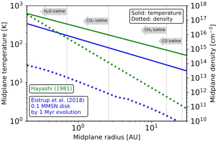
Fig. 1.Physical structures of disk midplanes for pre-solar nebula from Hayashi (1981) (in green), and for 0.1 MMSN disk by 1 Myr evolution from Eistrup et al. (2018) (in blue). Solid profiles are for temperature. Dotted profiles are for number density. The vertical grey lines indicate the positions of the icelines of H2O, CO2, CH4and CO by 1 Myr

evolu-tion for the 0.1 MMSN disk in Eistrup et al. (2018). The grey arrows on each of the vertical lines indicate which species each line is associated with, and how the iceline moves over time (all inwards).

istry in a protoplanetary disk midplane. The chemical modelling includes gas-phase chemistry, gas-interactions, and grain-surface (ice) chemistry. The gas-phase chemistry is from the latest release of the UMIST Database for Astrochemistry (see McElroy et al. 2013) termed Rate12, and the gas-grain

interac-tions and grain-surface chemistry are as described in Walsh et al. (2015), and references therein. The statistical method used is de-scribed in Section 2.2.

2.1. Model description

The modelled volatile ice abundances are taken from Eistrup et al. (2018). A physical disk model evolving in time was used featuring decreasing temperature and density structures from 0 to 30 AU, with the CO iceline residing inside 30 AU. Icelines (or snowlines) mark the radius in the disk midplane beyond which species exist solely in ice form and are thus depleted from the gas. This occurs at the radius where the accretion rate onto grain surfaces (or freezeout) exceeds the desorption rate from grain surfaces due to the negative temperature gradient in the midplane. The position of the midplane iceline for a particular species will depend on its volatility (that is, its binding energy).

The disk structure used is not the pre-solar nebula structure proposed by Hayashi (1981), and parameterised in Aikawa et al. (1997). However, the utilised disk structure here is evolving in time, and chemical evolution model results are readily available from Eistrup et al. (2018). Besides, the locations in the disk im-portant to comet formation are the volatile icelines, which are closer to the star for a colder disk, and further away from the star for a warmer disk. Tracking comet formation based on iceline positions therefore means that the exact choice of physical disk structure is less important, and in addition, the 30 AU range of this disk covers all important icelines (including the CO iceline which starts just inside 30 AU).

(3)

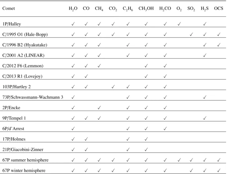
struc-Table 1.Molecules detected in each comets included in this work

Comet H₂O CO CH₄ CO₂ C₂H₆ CH₃OH H₂CO O₂ SO₂ H₂S OCS

1P/Halley X X X X X X X X X

C/1995 O1 (Hale-Bopp) X X X X X X X X X X

C/1996 B2 (Hyakutake) X X X X X X X X

C/2001 A2 (LINEAR) X X X X X X X

C/2012 F6 (Lemmon) X X X X X

C/2013 R1 (Lovejoy) X X X X

103P/Hartley 2 X X X X X X

73P/Schwassmann-Wachmann 3 X X X X X

2P/Encke X X X X X

9P/Tempel 1 X X X X X X X

6P/d’Arrest X X X X

17P/Holmes X X X X

21P/Giacobini-Zinner X X X X

67P summer hemisphere X X X X X X X X X X X

67P winter hemisphere X X X X X X X X X X

ture from Hayashi (1981) is warmer (roughly twice as high tem-perature at any radius) and more massive (more than ten times higher mass) compared to the disk from Eistrup et al. (2018) (hence the “0.1 Minimum Mass solar Nebula”-designation for this disk). It is noted that the disk from Eistrup et al. (2018) has already lost mass by 1 Myr evolution, so in Fig. 1 the density dif-ference between the disks is more than ten times. The disk mass of 0.1 MMSN from Eistrup et al. (2018) is the initial mass of the disk, not the mass by 1 Myr (as plotted in Fig. 1).

Results for the “high” ionisation rate are taken, which in-cludes contributions from galactic cosmic rays, as well as decay products of short-lived radionuclei in the disk midplane (see e.g. Cleeves et al. 2013; Padovani et al. 2018). A timescale up to 8 Myr is assumed for a long-lived gaseous protoplanetary disk. The high ionisation rate of typically 10−17_s−1_{means that}

chemi-cal changes occur after a few 105yrs. The disk structure cooling in time means that the volatile icelines move inwards in time.

Two different sets of initial abundances are assumed: inher-itance and reset. Inherinher-itance assumes all ices to have survived the trip from the parent molecular cloud to the disk midplane, thereby starting the chemical modelling with neutral molecules that are abundant in interstellar ices. The reset scenario assumes an energetic event to have dissociated all molecules into atoms (chemical reset) upon arrival in the midplane, thereby starting the chemical modelling with highly reactive atoms. Such a reset can occur for in-falling material that comes close to the proto-star in the earliest stages of disk formation (see e.g. Visser et al.

2009). The inner solar system is assumed to have undergone some amount of chemical reset (with evidence from studies of chondrules and CAIs, see e.g. Trinquier et al. 2009), followed by a condensation sequence, depending on location in the disk. Comets, on the other hand, are often thought to be pristine, pos-sibly because they formed, and mainly reside, in the outer solar system.

(4)

Daughter species in general have been excluded because the parent species are expected to be dominant in cometary ices, even if the daughter species are abundant in the comae. Since the daughter species in the coma originate from dissociated par-ent species in the gas after sublimation, the exclusion of daugh-ter species means that the detected abundances of parent species in the coma are likely lower than the actual abundance on the cometary surface.

The detected abundances of each molecule in each comet are taken from Tables 2, 3, 4, and 5 in Le Roy et al. (2015). If, for a given molecule in a given comet in these tables, multiple abundance values and/or ranges are given, then the smallest and the largest of these values (and/or range limits) are taken as the error range for the abundance of that molecule in that comet, and the average of the smallest and largest values is taken as the measured abundance of that molecule in that comet. Upper limit values, or upper limit ranges given in the tables in Le Roy et al. (2015) are considered non-detections, and are thus not included in the analysis. If only one abundance value is available for a molecule in a comet, then a conservative error estimate of 50% of the observed value is assumed. This estimate is reasonable when compared with observed errors (see right-hand panels of Figures A1 to A5).

In addition to these cometary abundance measurements, the abundance measurement of CO in comet 17P by Qi et al. (2015) is included, using a CO/HCN ratio of 40±5 as representative of the bulk cometary composition of comet 17P. The measured abundance of HCN relative to H₂O from Dello Russo et al. (2008) (HCN/H₂O=0.538 (%)) is then used to normalise the CO abundance in comet 17P to the H₂O abundance (assum-ing the aforementioned 50% error on the HCN/H₂O measure-ment). Propagating both the error on the measurement by Qi et al. (2015), and the 50% estimated error of the measurement by Dello Russo et al. (2008) leads to CO/H₂O=21.52±11.09 (%) for comet 17P, which is used in the analysis here. An overview of the comets included in the analysis is shown in Table 1, which also indicates which molecules have been measured in each comet.

It is noted that this work will refer to the different comets listed in Table 1, either by using theirP-identifiers (e.g. comets 2P, 9P, and 67P-W, where the extension “-W” indicates the win-ter hemisphere of comet 67P), or by their commonly used names, as listed in parentheses in Table 1 (e.g. comets Halley or Hyaku-take). Therefore, please refer to this table for the cometary body identifier codes.

2.2. Statistical comparison between observations and models

With observed abundances of several molecules available for all comets, along with the evolving spatial midplane abundances of those molecules, it can now be quantified how likely it is for a comet to have formed at a given time and place, assuming that the comets acquired all their ices at one time and place, and that the ices remained unaltered thereafter. For each comet, a log-spaceχ2-surface in timetand radiusris computed. We do the analysis in log-space because of the large dynamical range (or-ders of magnitude) in the modelled abundances; hence, we con-sider a good agreement to lie within an order of magnitude of the observed ratio. For each set of radiusrand timet, theχ2_value

for a given comet is given by

χ2₍_r,_t₎₌ n X

i=1

log(ni,obs(r,t))−log(ni,mod(r,t))2

σ0

i,obs(r,t)

2 , (1)

where ni,obs(r,t) and ni,mod(r,t) are the observed and mod-elled abundances of speciesi with respect to H₂O ice at (r,t).

σ0

i,obs(r,t) is defined as

σ0

i,obs(r,t)=0.434

σi,obs(r,t)

ni,obs(r,t) (2)

where σi,obs(r,t) is the observed or estimated error on the

abundance, and σ0_i,obs(r,t) is the propagated error appropriate when using the log-function.

The χ2_{-surface for each comet is then transformed into a}

maximum likelihood functionP(r,t) using

P(r,t)=e−χ2(r,t)/2 (3)

and subsequently all sets of P(r,t) for each comet are nor-malised by the maximum P-value for that comet. The result-ing surfaces of maximum likelihood show contours of different colours in different regions of parameter space, with colours de-pending on how close a region is to the maximum likelihood value for the comet. Regions of parameter space close to the maximum likelihood value for a comet are in turn the regions showing best agreement between the chemical models and the observed cometary abundances.

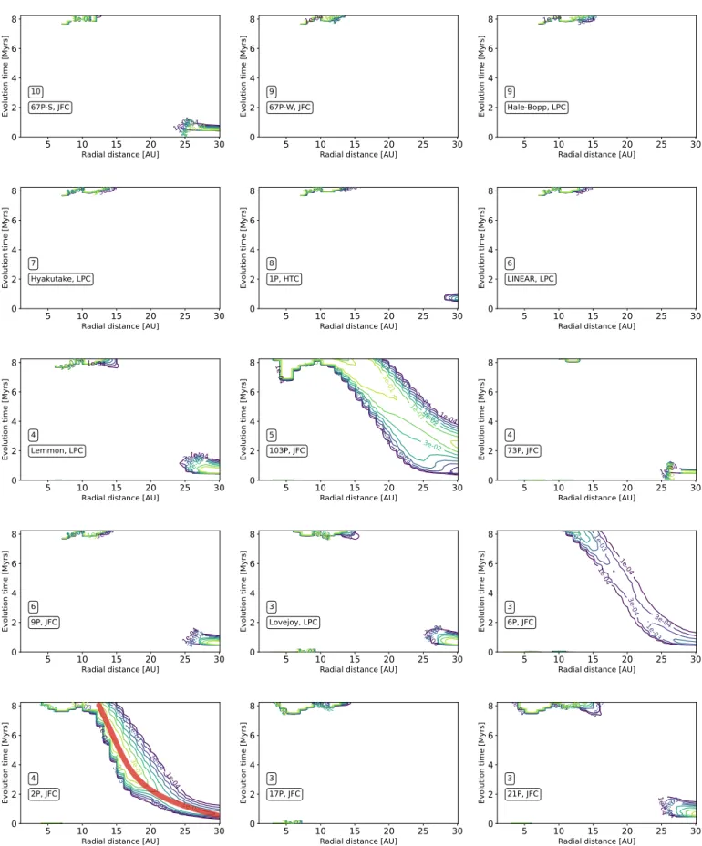
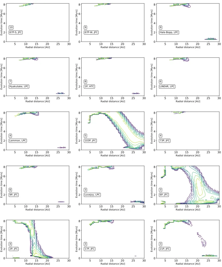
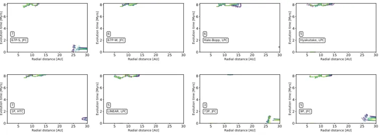
These maximum likelihood (P-value) surfaces are shown for all comets in Fig. 2, which compares observations with models of the reset scenario, and in Fig. 3 for models of the inheritance scenario. Thex-axes in each panel in each figure are radial dis-tance from the star in AU, and they-axes are chemical evolution time in Myr. For each contour level the value of the contour indi-cates where the fraction of the localP-value to the maximumP -value is above a certain level, for each comet. Regions of yellow contour indicate good agreement between models and observa-tions, whereas darker colours indicate poorer agreements.

The comet names, and dynamical types from Cochran et al. (2012), are listed in all panels. In each panel is also given the number of molecular detections for each comet (from Le Roy et al. 2015), with the panels from left to right, and top to bottom featuring decreasing numbers of molecular detections per comet. This way, the first panel with ten molecular detections (Comet 67P-S) can be distinguished from the last panel with only two molecular detections (Comet 21P), in that more molecular de-tections in a comet should make the comparison between the models and the observations more robust.

3. Results

3.1. Full sample of species: reset scenario

(5)

red shaded region overplotted for comet 2P, and this trail over-laps with the regions of highest likelihood for all comets.

This trail, in turn, roughly traces the vicinity of the CO ice-line (atT ∼21 K), as is seen in the left panel of Fig. 4 in Eistrup et al. (2018). That figure, amongst others, shows the changing lo-cation of the CO iceline in the physically evolving disk midplane utilised in that work. This is interesting, because it points to all the comets here agreeing well with formation in the vicinity of the CO iceline in the pre-solar nebula. Additionally, all comets show high likelihood of formation at 6-13 AU by 7-8 Myr, a range encompassing also the CH₄ iceline (see again Fig. 4, left panel, in Eistrup et al. 2018).

Comet 103P is the only comet showing some likelihood of formation at ∼30 AU by 2-3 Myr of evolution. However, the maximum likelihood of formation for this comet is at 10-15 AU by∼8 Myr, which is consistent with the rest of the comets.

3.2. Full sample of species: inheritance scenario

Turning to the inheritance scenario the maximum likelihood sur-faces for all comets are presented in Fig. 3. All comets in this scenario share good agreement with formation at ∼12 AU by 8 Myr, similar to the case for the reset scenario in Fig. 2. All comets also show agreement with late formation (7-8 Myr) from small radii out to 10 AU, and some (103P, 6P, Lovejoy and 21P) also agree well with having formed inside 5 AU at various times during the evolution. The trail along the CO iceline that was seen for the reset scenario is not reproduced for all comets in the inheritance scenario. However, Hale-Bopp, LINEAR, Lemmon, 103P, 9P, 6P, and 21P do somewhat agree with parts of the trail (103P and 6P are both in good agreement with the trail). Most of the comets for the inheritance scenario also agree with formation at 25-30 AU by<1 Myr evolution. However, the best agreements between models and observations are for late evolutionary times. Lastly, addressing both the reset scenario in Fig. 2 and the inheritance scenario in Fig. 3 it is generally seen that the more species that are observed in a comet (the top panels of each fig-ure), the smaller the regions in parameter space over which the models well reproduce the observed ratios, thus better constrain-ing the potential formation location and time of formation.

3.3. Correlation for C- and O-carrying species only

Given the interlinked chemical nature of carbon and oxygen, and the fact that the modelled nitrogen and sulphur chemistry is less well understood, it is interesting to have a look at maximum like-lihood surfaces for the comets excluding sulphur species, and considering only ice species with carbon and oxygen. In the sam-ple of molecules from Le Roy et al. (2015) these species are: C₂H₆, CO₂, CO, H₂CO, CH₃OH, CH₄, and O₂, thus seven in total.

For these seven ice species maximum likelihood surfaces are shown in Fig. 4 for the reset scenario and in Fig. 5 for the inher-itance scenario. Since sulphur species have only been observed for comets 1P, Hale-Bopp, Hyakutake, LINEAR, 73P, 9P, and 67P (both seasons), only these comets are relevant to analyse for differences compared to the analysis with the full sample of species.

Comparing these maximum likelihood surfaces to their counterparts in Fig. 2 for the reset scenario and Fig. 3 for the inheritance scenario reveals that excluding sulphur species does not significantly change the behaviour in the results. The only apparent difference is found for comet Hale-Bopp, which in the

reset scenario in Fig. 4 without sulphur agrees more broadly with formation at various evolutionary times and locations (though still along the CO iceline) than it did when including sulphur. However, this makes sense because excluding species from the analysis should cause less constraints on the most likely time and location of formation.

4. Discussion

Studies of comets and cometary compositions so far have been grouping them by either dynamical characteristics (length of or-bit or inclination), or by their molecular contents (see Cochran et al. 2012). A’Hearn et al. (1995) and Cochran et al. (2012) de-fined standards for molecular abundances (typical or depleted), such that cometary measurements could then indicate either en-hanced or depleted abundances for a given molecule. While this approach does provide a grouping for comets that fit with the standard, it fails to include the possible chemical evolution of the comet-forming material in setting that standard.

This work attempts to trace the formation histories of 15 comets, by comparing cometary abundances with evolving ice abundances in a protoplanetary disk midplane through statisti-cal tests. This way, rather than simply comparing similarities in the cometary contents, the potential formation times of the comets can also be addressed, since the chemical composition of the comet-forming disk midplane evolves over time. Four diff er-ent comparison setups were investigated, with two different sets of observed abundances (either including or excluding sulphur-bearing species), and two different models for evolving abun-dances for the midplane (the inheritance or the reset scenario). For the reset scenario, good agreement is seen for formation in the vicinity of the CO iceline for all 15 comets.

The comets with more species observed in the coma are con-strained to either formation at 27-30 AU by∼1 Myr evolution, or to formation at∼12 AU by 8 Myr evolution. Comets with fewer observed species agree well with formation along the CO iceline, as indicated by the red shaded region overplotted on the panel for comet 2P in Fig. 2. From the left panel in Fig. 4 from Eistrup et al. (2018), 30 AU is by 0.5 Myr just outside the CO iceline (at 27 AU), which moves to 12 AU by 8 Myr. The CH₄ iceline is found at 10 AU by 8 Myr. This suggests that for all comets, their formations can be constrained to lie roughly between the icelines of CH₄and CO, with some degeneracy remaining in the formation time. It is noted that comet 17P does not follow the trend for formation between the CO and CH₄icelines, unless the CO abundance measured by Qi et al. (2015) is included in the analysis.

For the inheritance scenario, both with and without sulphur-bearing species, the results do not point as strongly to formation along the CO iceline, as found for the reset scenario. There is a similarity between the reset and inheritance scenarios with good agreement for formation at 11-13 AU by 8 Myr, but this should be seen in the light of the results from Eistrup et al. (2018). It is shown there that the ice abundances for both scenarios tend towards icy disk midplane steady state at late evolutionary times (>5 Myr). That means that the ice abundances after 5 Myr evo-lution are largely similar across the two scenarios, resulting in similar maximum likelihood surfaces for both (see also the abun-dance evolution surfaces in Figs A.1 -A.5).

(6)

5 10 15 20 25 30 Radial distance [AU]

0 2 4 6 8

Evolution time [Myrs] 67P-S, JFC 10 1e-04 1e-04 3e-04 3e-04 1e-03 1e-03 3e-03 3e-03 1e-02 1e-02 3e-02 3e-02 1e-01 1e-01 3e-01 3e-01

5 10 15 20 25 30

Radial distance [AU] 0

2 4 6 8

Evolution time [Myrs] 67P-W, JFC 9

1e-043e-011e-013e-021e-023e-041e-033e-03

5 10 15 20 25 30

2 4 6 8

Evolution time [Myrs] Hale-Bopp, LPC 9

1e-04 3e-04 1e-03 3e-011e-013e-021e-023e-03

5 10 15 20 25 30

2 4 6 8

Evolution time [Myrs] Hyakutake, LPC 7

1e-04 3e-04

1e-03 3e-03

1e-02 3e-02 3e-011e-01

5 10 15 20 25 30

2 4 6 8

Evolution time [Myrs] 1P, HTC 8

1e-04

3e-04 1e-033e-03 1e-02 3e-02 1e-01

3e-01

5 10 15 20 25 30

2 4 6 8

Evolution time [Myrs] LINEAR, LPC 6 1e-04 3e-04 1e-03 3e-03 1e-02 3e-02 1e-01 3e-01

5 10 15 20 25 30

2 4 6 8

Evolution time [Myrs] Lemmon, LPC 4 1e-04 1e-04 3e-04 3e-04 1e-03 1e-03 3e-03 3e-03 1e-02 1e-02 3e-02 3e-02 1e-01 3e-01

5 10 15 20 25 30

2 4 6 8

Evolution time [Myrs] 103P, JFC 5 1e-04 1e-04 3e-04 3e-04 1e-03 1e-03 3e-03 3e-03 1e-02 1e-02 3e-02 3e-02 1e-01 1e-01 3e-01

5 10 15 20 25 30

2 4 6 8

Evolution time [Myrs] 73P, JFC 4

1e-04_3e-04_3e-03_1e-03_1e-023e-01_3e-02_1e-01

5 10 15 20 25 30

2 4 6 8

Evolution time [Myrs] 9P, JFC 6 1e-04 1e-04 3e-04 3e-04 1e-03 1e-03 3e-03 3e-03 1e-02 3e-021e-013e-01

5 10 15 20 25 30

2 4 6 8

Evolution time [Myrs] Lovejoy, LPC 3 1e-04 1e-04 1e-04 3e-04 3e-04 3e-04 1e-03 1e-03 1e-03 3e-03 3e-03 3e-03 1e-02 1e-02 3e-02 3e-02 1e-01 1e-01 3e-01 3e-01

5 10 15 20 25 30

2 4 6 8

Evolution time [Myrs] 6P, JFC 3 1e-04 1e-04 3e-04 3e-04 1e-03 1e-03 3e-03

5 10 15 20 25 30

2 4 6 8

Evolution time [Myrs] 17P, JFC 3 1e-04 1e-04 3e-04 3e-04 1e-03 1e-03 3e-03 3e-03 1e-02 1e-02 _1e-02 3e-02 3e-02 _3e-02 1e-01 1e-01 3e-01 3e-01

5 10 15 20 25 30

2 4 6 8

Evolution time [Myrs] 21P, JFC 3 1e-04 1e-04 3e-04 3e-04 1e-03 1e-03 3e-03

3e-03_3e-023e-01_1e-021e-01

Fig. 2.Maximum likelihood surfaces for reset scenario, for full sample of molecular species. The maximum likelihood increases from dark purple contours to light green contours. Darkest purple contour represents maximum likelihood of 10−4_{, and increases with each lighter contour level to}

3x10−4_{, 10}−3_{, 3x10}−3_{, 10}−2_{, 3x10}−2_{, 10}−1_{, and finally 3x10}−1_{for the lightest green contour. Radius in AU in the physically evolving protoplanetary}

(7)

5 10 15 20 25 30 Radial distance [AU]

0 2 4 6 8

Evolution time [Myrs] 67P-S, JFC 10

1e-04

3e-04

1e-033e-031e-023e-02

1e-01 3e-01

5 10 15 20 25 30

2 4 6 8

Evolution time [Myrs] 67P-W, JFC 9 1e-04 3e-04 1e-03 3e-03 1e-02 3e-021e-01 3e-01

5 10 15 20 25 30

2 4 6 8

Evolution time [Myrs] Hale-Bopp, LPC 9 1e-04 1e-04 3e-04 3e-04 1e-03 1e-03 3e-03 3e-03 1e-02 1e-02 3e-02 3e-02 1e-01 3e-01

5 10 15 20 25 30

2 4 6 8

Evolution time [Myrs] Hyakutake, LPC 7 1e-04 1e-04 3e-04 3e-04 1e-03 1e-03 3e-03 1e-02 3e-02 1e-01 3e-01

5 10 15 20 25 30

2 4 6 8

Evolution time [Myrs] 1P, HTC 8

1e-04

1e-04 3e-041e-033e-031e-023e-021e-013e-01

5 10 15 20 25 30

2 4 6 8

Evolution time [Myrs] LINEAR, LPC 6

1e-04 _3e-04

1e-03

3e-03

1e-023e-021e-01

3e-01

5 10 15 20 25 30

2 4 6 8

Evolution time [Myrs] Lemmon, LPC 4

1e-04

1e-04 3e-04

1e-031e-023e-03 1e-013e-02

3e-01

5 10 15 20 25 30

2 4 6 8

Evolution time [Myrs] 103P, JFC 5 1e-04 1e-04 3e-04 3e-04 1e-03 1e-03 3e-03 3e-03 1e-02 1e-02 3e-02 3e-02 1e-01 1e-01 3e-01 3e-01

5 10 15 20 25 30

2 4 6 8

Evolution time [Myrs] 73P, JFC 4 1e-04 3e-04 1e-03 3e-03 1e-02 3e-02 1e-01 3e-01

5 10 15 20 25 30

2 4 6 8

Evolution time [Myrs] 9P, JFC 6 1e-04 3e-04 1e-03 3e-03 1e-02 3e-02 1e-013e-01

5 10 15 20 25 30

2 4 6 8

Evolution time [Myrs] Lovejoy, LPC 3 1e-04 1e-04 3e-04 3e-04 1e-03 1e-03 3e-03 3e-03 1e-02 1e-02

3e-021e-013e-01

5 10 15 20 25 30

2 4 6 8

Evolution time [Myrs] 6P, JFC

3 1e-04

1e-04

3e-04

3e-04 3e-04 1e-03

1e-03 1e-03 3e-03 3e-03 3e-03 1e-02 1e-02 1e-02 3e-02 3e-02 3e-02 1e-01 1e-01 1e-01 1e-01 3e-01 3e-01 3e-01 3e-01

5 10 15 20 25 30

2 4 6 8

Evolution time [Myrs] 2P, JFC 4 1e-04 3e-04 1e-03 3e-03 1e-02 3e-02 3e-02 1e-01 1e-01 3e-01 3e-01

5 10 15 20 25 30

2 4 6 8

Evolution time [Myrs] 17P, JFC 3 1e-04 1e-04 3e-04 3e-04 1e-03 1e-03 3e-03 3e-03 1e-02 1e-02 3e-02 3e-02 1e-01 1e-01 3e-01 3e-01

5 10 15 20 25 30

2 4 6 8

Evolution time [Myrs] 21P, JFC 3 1e-04 1e-04 1e-04 3e-04 3e-04 1e-03 1e-03 3e-03 3e-03 1e-02 1e-02 3e-02 3e-02 3e-02 1e-01 1e-01 1e-01 3e-01 3e-01 3e-01

Fig. 3.Maximum likelihood surfaces for inheritance scenario, for full sample of molecular species. The maximum likelihood increases from dark purple contours to light green contours. Darkest purple contour represents maximum likelihood of 10−4_{, and increases with each lighter contour}

level to 3x10−4_{, 10}−3_{, 3x10}−3_{, 10}−2_{, 3x10}−2_{, 10}−1_{, and finally 3x10}−1 _{for the lightest green contour. Radius in AU in the physically evolving}

(8)

5 10 15 20 25 30

Radial distance [AU]

0 2 4 6 8

Evolution time [Myrs] 67P-S, JFC

7 1e-04 1e-04 3e-04 3e-04 1e-03 1e-03 3e-03 3e-03 1e-02 1e-02 3e-02 1e-01 3e-01

5 10 15 20 25 30

0 2 4 6 8

Evolution time [Myrs] 67P-W, JFC

6 1e-04

3e-04

1e-03

3e-033e-013e-021e-011e-02

5 10 15 20 25 30

0 2 4 6 8

Evolution time [Myrs] Hale-Bopp, LPC

6 1e-04 3e-04 1e-03 3e-03 1e-02 3e-02 1e-01 3e-01

5 10 15 20 25 30

0 2 4 6 8

Evolution time [Myrs] Hyakutake, LPC

5

1e-04_1e-01_1e-03_3e-03_1e-02_3e-02_3e-01_3e-04

5 10 15 20 25 30

0 2 4 6 8

Evolution time [Myrs] 1P, HTC

7

1e-04 3e-04 1e-03 3e-013e-021e-013e-031e-02

5 10 15 20 25 30

0 2 4 6 8

Evolution time [Myrs] LINEAR, LPC

5 1e-04 3e-04 1e-03 3e-03 1e-02 3e-02 1e-013e-01

5 10 15 20 25 30

0 2 4 6 8

3

1e-043e-041e-033e-031e-023e-021e-01 3e-01

5 10 15 20 25 30

0 2 4 6 8

5 1e-04 1e-04 3e-04 3e-04 1e-03 1e-03 3e-03 3e-03 1e-02 3e-02 1e-01 3e-01

Fig. 4.Maximum likelihood surfaces for reset scenario, considering C- and O-bearing species only. The maximum likelihood increases from dark purple contours to light green contours. Darkest purple contour represents maximum likelihood of 10−4_{, and increases with each lighter contour}

level to 3x10−4_{, 10}−3_{, 3x10}−3_{, 10}−2_{, 3x10}−2_{, 10}−1_{, and finally 3x10}−1 _{for the lightest green contour. Radius in AU in the physically evolving}

protoplanetary disk midplane is on thex-axis, and evolution time in Myrs is on they-axis.

5 10 15 20 25 30

0 2 4 6 8

Evolution time [Myrs] 67P-S, JFC

7 1e-043e-041e-033e-03

1e-02

3e-02 1e-01 3e-01

5 10 15 20 25 30

0 2 4 6 8

Evolution time [Myrs] 67P-W, JFC

6 1e-04 3e-04 1e-03 3e-03 1e-02 3e-02 1e-01 3e-01

5 10 15 20 25 30

0 2 4 6 8

Evolution time [Myrs] Hale-Bopp, LPC

6 1e-04 1e-04 3e-04 3e-04 1e-03 1e-03 3e-03 3e-03 1e-02 1e-02 3e-02 3e-02 1e-013e-01

5 10 15 20 25 30

0 2 4 6 8

Evolution time [Myrs] Hyakutake, LPC

5 1e-04 1e-04 3e-04 3e-04 1e-03 1e-03 3e-03 1e-02 3e-02 1e-01 3e-01

5 10 15 20 25 30

0 2 4 6 8

Evolution time [Myrs] 1P, HTC

7 1e-04 1e-04 3e-04 1e-03 3e-03 1e-02 3e-021e-013e-01

5 10 15 20 25 30

0 2 4 6 8

Evolution time [Myrs] LINEAR, LPC

5 1e-04 _3e-04 1e-03 3e-03 1e-02 3e-02 1e-013e-01

5 10 15 20 25 30

0 2 4 6 8

3

1e-04 3e-04 1e-03 3e-03 1e-02 3e-021e-013e-01

5 10 15 20 25 30

0 2 4 6 8

5 1e-04 3e-04 1e-03 3e-03 1e-02 3e-02 1e-013e-01

Fig. 5.Maximum likelihood surfaces for inheritance scenario, considering C- and O-bearing species only. The maximum likelihood increases from dark purple contours to light green contours. Darkest purple contour represents maximum likelihood of 10−4_{, and increases with each lighter}

contour level to 3x10−4_{, 10}−3_{, 3x10}−3_{, 10}−2_{, 3x10}−2_{, 10}−1_{, and finally 3x10}−1_{for the lightest green contour. Radius in AU in the physically evolving}

(9)

that our starting molecular abundances for the inheritance sce-nario do not resemble well those for the particular molecular cloud from which the Sun formed. Although this set of abun-dances are motivated by observations of ices in protostellar (or interstellar) environments (see Eistrup et al. 2016), it is possi-ble that the Sun formed in a different (warmer) environment to that for nearby well-studied protostellar sources (see e.g. Adams 2010; Taquet et al. 2018). It would be worthwhile to explore the impact of a warmer interstellar environment on the initial inher-ited molecular abundances for a comet-forming disk.

Using the analysis here as a test of which chemical starting conditions and evolution best agree with the observations, the reset scenario is seen to generally agree best with the cometary observation, by constraining all the comets to most likely having formed between the icelines of CH₄ and CO. As these icelines reside at temperatures (TCO,ice ∼ 21K and TCH₄,ice ∼ 28K) at which grain-surface (ice) chemistry is particularly active, large changes in the relative abundances of the volatile ice species are seen over time (see Eistrup et al. 2018). This active chemistry could in turn explain the diversity of observed cometary abun-dances.

That the reset scenario provides better constraints on location and time for comet formation, points to the comet-forming re-gion in the pre-solar nebula having been seeded with chemically processed material. This chemical processing can have several origins including an accretion shock en routeinto the forming disk, turbulent mixing within the disk once formed, or an accre-tion outburst caused by material in-falling from the disk onto the star. If any (all) of these processes have occurred, then this sup-ports an early formation of comets (<1 Myr). However, if the pre-solar nebula formed and evolved in a quiescent manner, a late formation of comets (∼8 Myr) is also supported. In this lat-ter case, it cannot be distinguished whether or not the cometary material has an interstellar origin.

Addressing the formation times of the comets also leads to the question of whether or not each individual comet formed quickly (e.g. assembly took place within 0.5 Myr after the comet started forming), or if each comet formed slowly, such that its assembly could have lasted throughout the lifetime of the pre-solar nebula disk midplane. In the former case, a quick assem-bly of the icy material at a given radius into a larger cometary body could have acted to impede chemical processing of the ices inside the comet, such that the composition inside the comet would remain unaltered, representing the composition of the icy material at the specific time and radius at which the assembly took place in the disk midplane. In the latter case, on the other hand, if the comet assembled slowly during the lifetime of the pre-solar nebula disk midplane, then the solid material incorpo-rated into the comet would have experienced different degrees of chemical evolution in the disk midplane, and hence have dif-ferent ice compositions, depending on what time that material was incorporated into the comet. Assuming again that, subse-quent to the comet’s final assembly, the ice chemistry inside it is impeded, then the observed cometary abundances in this slowly-formed comet would likely be a mix of different, say, H₂O ice abundances from different times during its formation. When ob-served, such a possible mix of different abundances of one ice species inside the comet would then likely manifest as the aver-age over these different abundances, thereby not carrying a fin-gerprint of any specific time and radius of formation. The results presented here highlight specific formation times and radii for individual comets which suggests that quick assembly of comets is possible. However, further calculations are needed to ascertain

to what degree a slower rate of assembly can influence the bulk comet composition over time.

Comparing the grouping of 15 comets here with the previous cometary classifications from Cochran et al. (2012) as typical, depleted or “mixed classification” (as of Table 2 in Le Roy et al. 2015) they fall under all these three classes. These 14 comets have thus never been grouped chemically together before. With these 14 comets now grouped together based on likely formation in the vicinity of the CO iceline, it is also possible to propose a formation sequence for this group, based on the peak of the maximum likelihood surface for each comet in Fig. 2.

Based on this, the following formation time classes from early to late for the 15 comets can be proposed: 9P, 73P, Lem-mon, and Lovejoy (all comets feature maximum likelihood peaks from 0.4-0.64 Myr at 28-30 AU), 2P (by 4.3 Myr at 16 AU), and 1P, 6P, 17P, 21P, 67P-S, 67P-W, 103P, Hyakutake, LINEAR, and Hale-Bopp (by 8.23 Myr at 11-13 AU). It is noted that some of these comets have their maximum likelihood peaks located outside of the formation region around the CO iceline. For the sake of focusing on the possible formation time classification around this iceline, only likelihood peaks happening between 0.4 and 8.23 Myr were used for the analysis, thereby ignoring peaks outside of the CO iceline region of the parameter space. This formation time classification creates one group of four comets that possibly formed early, between 0.4-0.64 Myr, one comet that possibly formed at an intermediate time by 4.3 Myr, and another group of ten comets that possibly formed later after 8 Myr. This hints that comet formation may occur in tandem with disk evolution over∼8 Myr timescales.

This formation classes should be considered in light of which comets have more detections. As is evident in Fig. 2, the max-imum likelihood peaks are very localised (either∼13 AU by 8 Myr or at∼30 AU by 1 Myr) for the comets that have more de-tections. The comets with fewer detections are less constrained and thus have larger regions of parameter space with good agree-ment with the models. The comets with more detections are thus constrained to having formation times similar to each other.

An interesting additional consideration regards which spe-cific species have been detected in which comets, and how that may relate to which regions of parameter space the comets are in best agreement with. Comets 73P, 2P, and 6P have no CO detec-tions in them, yet in the analysis here these are all constrained to have formed in the vicinity of the CO iceline. Detection of CO in a comet is thus not a pre-requisite for constraining the comet for-mation (roughly) to this region. It is noted that a comet that has formed inside of the CO ice line should naturally be CO poor.

(10)

to a different species that is less susceptible to summer and win-ter effects.

5. Conclusion

In this work a statisticalχ2method has been used to perform a quantitative comparison between observed cometary abundances and modelled chemical evolution in a protoplanetary disk mid-plane, by computing maximum likelihood surfaces, as a function of disk midplace location (radius) and time. The best agreements between observed and modelled abundances were found when considering the chemical evolution models to be chemically re-set at the start, thus assuming that the volatile content of the pre-solar nebula was (perhaps partially) atomised before dust grains starting building larger bodies. This is consistent with the tradi-tional idea about the chemical start of the inner pre-solar nebula (Grossman 1972), but not the outer nebula.

All 15 comets (14, when counting 67P-W and 67P-S as one) were found to have high likelihoods of formation along a trail in time and radial parameter space which is in the vicinity of the CO iceline. Since CO is the molecule (next to N₂ and H₂) with the lowest binding energy (Eb=855 K) this means that most molecules are in the ice at the point where the comets are most likely to have formed. We do not consider formation radii here that are outside of the CO iceline, as the abundances in this re-gion are found to be very different from those around the iceline (see Eistrup et al. 2018). There, it is found that the grain-surface chemistry is mainly driven by hydrogenation reactions leading to high abundances of, for example, H₂O, CH₄, C₂H₆, and CH₃OH ices.

Based on the maxima of the likelihood functions for each comet along the CO iceline, it was then determined when during chemical evolution each comet was most likely to have formed. Thereby a formation time classification for all 15 comets was proposed, with some degeneracy remaining between the early (<1 Myr) and late (>7.5 Myr) formation. With more samples of comets with sufficient molecular detections in the future, it will be possible to further test this chemical evolution classification scheme for formation histories of comets. It will be interesting to see if other comets support the idea of a chemical reset start, and if they too show best agreement with formation in the vicinity of the CO iceline.

Acknowledgements. This work was motivated by discussions at the International

Space Science Institute in Bern during meetings of International Team 361, “From Qualitative to Quantitative: Exploring the Early solar system by Connect-ing Comet Composition and Protoplanetary Disk Models”, led by Dr Boncho Bonev. The authors thank the anonymous referee for valuable comments and input that helped improve the manuscript, and for pointing out the published measurements of CO in comet 17P, which led to the inclusion of the CO abun-dance for this comet. C.E. also thanks Chunhua Qi for discussions and sugges-tions on which measured CO abundance value to use for comet 17P in this work, and Anita Cochran for an interesting discussion. Astrochemistry in Leiden is supported by the European Union A-ERC grant 291141 CHEMPLAN and the Netherlands Research School for Astronomy (NOVA). C.W. acknowledges sup-port from the University of Leeds and the Science and Technology Facilities Council (grant No. ST/R000549/1). C.E. acknowledges the Virginia Initiative on Cosmic Origins (VICO) Fellowship for financial support.

References

Adams, F. C. 2010, ARA&A, 48, 47

A’Hearn, M. F., Millis, R. C., Schleicher, D. O., Osip, D. J., & Birch, P. V. 1995, Icarus, 118, 223

Aikawa, Y., Umebayashi, T., Nakano, T., & Miyama, S. M. 1997, ApJ, 486, L51 Altwegg, K., Balsiger, H., & Geiss, J. 1994, A&A, 290, 318

Biver, N., Bockelée-Morvan, D., Boissier, J., et al. 2007, Icarus, 187, 253

Biver, N., Bockelée-Morvan, D., Crovisier, J., et al. 1999, AJ, 118, 1850 Biver, N., Bockelée-Morvan, D., Crovisier, J., et al. 2008, in Asteroids, Comets,

Meteors 2008, Vol. 1405, 8149

Biver, N., Bockelée-Morvan, D., Crovisier, J., et al. 2006, A&A, 449, 1255 Biver, N., Bockelée-Morvan, D., Debout, V., et al. 2014, A&A, 566, L5 Bockelée-Morvan, D., Biver, N., Crovisier, J., et al. 2014, A&A, 562, A5 Bockelée-Morvan, D., Brooke, T. Y., & Crovisier, J. 1995, Icarus, 116, 18 Bockelée-Morvan, D., Crovisier, J., Mumma, M. J., & Weaver, H. A. 2004, The

composition of cometary volatiles, 391–423

Bockelée-Morvan, D., Debout, V., Erard, S., et al. 2015, A&A, 583, A6 Bockelée-Morvan, D., Lis, D. C., Wink, J. E., et al. 2000, A&A, 353, 1101 Brooke, T. Y., Tokunaga, A. T., Weaver, H. A., et al. 1996, Nature, 383, 606 Cleeves, L. I., Adams, F. C., & Bergin, E. A. 2013, ApJ, 772, 5

Cochran, A. L., Barker, E. S., & Gray, C. L. 2012, Icarus, 218, 144 Colangeli, L., Epifani, E., Brucato, J. R., et al. 1999, A&A, 343, L87 Combes, M., Moroz, V. I., Crovisier, J., et al. 1988, Icarus, 76, 404

Dello Russo, N., Mumma, M. J., DiSanti, M. A., Magee-Sauer, K., & Novak, R. 2001, Icarus, 153, 162

Dello Russo, N., R. J. Vervack, J., Weaver, H. A., et al. 2008, The Astrophysical Journal, 680, 793

Dello Russo, N., Vervack, R. J., J., Lisse, C. M., et al. 2011, ApJ, 734, L8 Dello Russo, N., Vervack, R. J., J., Weaver, H. A., et al. 2009, ApJ, 703, 187 Dello Russo, N., Vervack, R. J., Weaver, H. A., et al. 2007, Nature, 448, 172 Despois, D., Biver, N., Bockelée-Morvan, D., & Crovisier, J. 2005, in IAU

Sym-posium, Vol. 231, Astrochemistry: Recent Successes and Current Challenges, ed. D. C. Lis, G. A. Blake, & E. Herbst, 469–478

DiSanti, M. A., Anderson, W. M., Villanueva, G. L., et al. 2007a, ApJ, 661, L101 DiSanti, M. A., Mumma, M. J., Dello Russo, N., Magee-Sauer, K., & Griep,

D. M. 2003, Journal of Geophysical Research (Planets), 108, 5061 DiSanti, M. A., Villanueva, G. L., Bonev, B. P., et al. 2007b, Icarus, 187, 240 Eberhardt, P. 1999, Space Sci. Rev., 90, 45

Eberhardt, P., Meier, R., Krankowsky, D., & Hodges, R. R. 1994, A&A, 288, 315

Eistrup, C., Walsh, C., & van Dishoeck, E. F. 2016, A&A, 595, A83 Eistrup, C., Walsh, C., & van Dishoeck, E. F. 2018, A&A, 613, A14 Fink, U. 2009, Icarus, 201, 311

Gibb, E. L., DiSanti, M. A., Magee-Sauer, K., et al. 2007, Icarus, 188, 224 Gibb, E. L., Mumma, M. J., Dello Russo, N., DiSanti, M. A., & Magee-Sauer,

K. 2003, Icarus, 165, 391

Grossman, L. 1972, Geochim. Cosmochim. Acta, 36, 597

Hayashi, C. 1981, Progress of Theoretical Physics Supplement, 70, 35 Kawakita, H., Kobayashi, H., Dello Russo, N., et al. 2013, Icarus, 222, 723 Krankowsky, D., Lammerzahl, P., Herrwerth, I., et al. 1986, Nature, 321, 326 Le Roy, L., Altwegg, K., Balsiger, H., et al. 2015, A&A, 583, A1

Lis, D. C., Keene, J., Young, K., et al. 1997, Icarus, 130, 355

Magee-Sauer, K., Mumma, M. J., DiSanti, M. A., et al. 2008, Icarus, 194, 347 McElroy, D., Walsh, C., Markwick, A. J., et al. 2013, A&A, 550, A36 McPhate, J. B., Feldman, P. D., Weaver, H. A., et al. 1996, in AAS/Division

for Planetary Sciences Meeting Abstracts #28, AAS/Division for Planetary Sciences Meeting Abstracts, 09.29

Mumma, M. J., Bonev, B. P., Villanueva, G. L., et al. 2011, ApJ, 734, L7 Mumma, M. J. & Charnley, S. B. 2011, ARA&A, 49, 471

Mumma, M. J., Disanti, M. A., dello Russo, N., et al. 1996, Science, 272, 1310 Mumma, M. J., DiSanti, M. A., Dello Russo, N., et al. 2003, Advances in Space

Research, 31, 2563

Mumma, M. J., DiSanti, M. A., Dello Russo, N., Magee-Sauer, K., & Rettig, T. W. 2000, ApJ, 531, L155

Mumma, M. J., DiSanti, M. A., Magee-Sauer, K., et al. 2005, Science, 310, 270 Ootsubo, T., Kawakita, H., Hamada, S., et al. 2012, ApJ, 752, 15

Padovani, M., Ivlev, A. V., Galli, D., & Caselli, P. 2018, A&A, 614, A111 Paganini, L., DiSanti, M. A., Mumma, M. J., et al. 2014, AJ, 147, 15

Qi, C., Hogerheijde, M. R., Jewitt, D., Gurwell, M. A., & Wilner, D. J. 2015, ApJ, 799, 110

Radeva, Y. L., Mumma, M. J., Villanueva, G. L., et al. 2013, Icarus, 223, 298 Rubin, M., Tenishev, V. M., Combi, M. R., et al. 2011, Icarus, 213, 655 Schwarz, K. R. & Bergin, E. A. 2014, ApJ, 797, 113

Taquet, V., van Dishoeck, E. F., Swayne, M., et al. 2018, A&A, 618, A11 Trinquier, A., Elliott, T., Ulfbeck, D., et al. 2009, Science, 324, 374 Villanueva, G. L., Bonev, B. P., Mumma, M. J., et al. 2006, ApJ, 650, L87 Visser, R., van Dishoeck, E. F., Doty, S. D., & Dullemond, C. P. 2009, A&A,

495, 881

Walsh, C., Nomura, H., & van Dishoeck, E. 2015, A&A, 582, A88 Weaver, H. A., Chin, G., Bockelée-Morvan, D., et al. 1999, Icarus, 142, 482 Weaver, H. A., Feldman, P. D., A’Hearn, M. F., Dello Russo, N., & Stern, S. A.

2011, ApJ, 734, L5

Weaver, H. A., Feldman, P. D., McPhate, J. B., et al. 1994, ApJ, 422, 374 Woodney, L. M., McMullin, J., & A’Hearn, M. F. 1997, Planetary and Space

(11)

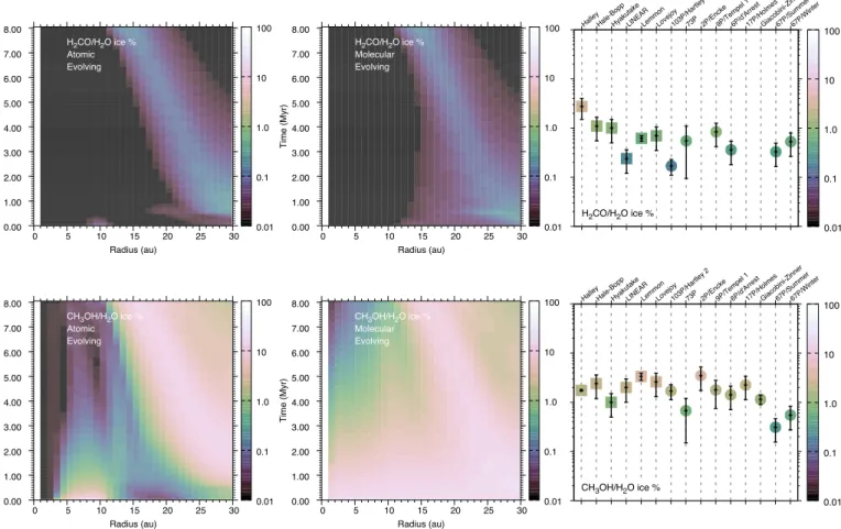
Appendix A: Evolving modelled abundances and cometary abundances

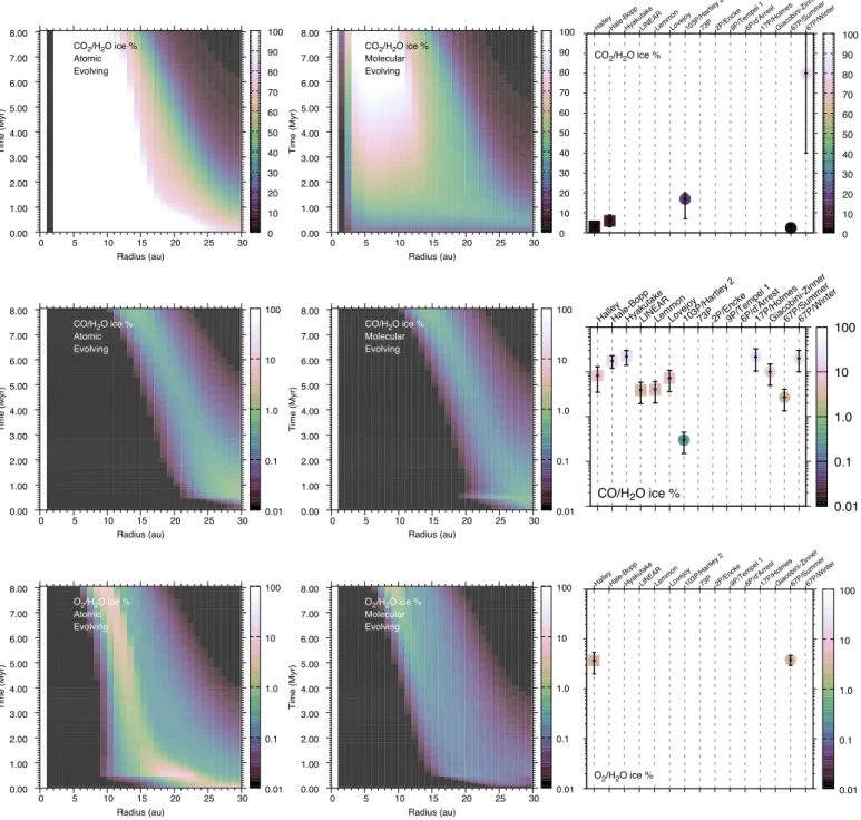
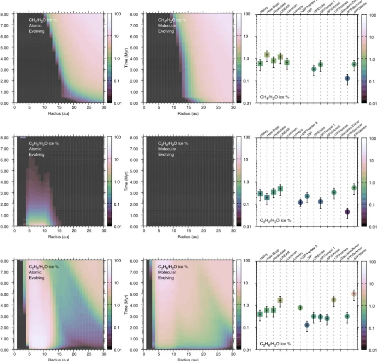
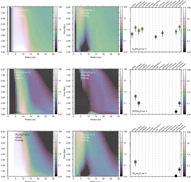
This appendix features abundance ratio maps (Figs. A.1-A.5) in radius and time for the molecular species considered in this work, as well as HCN, NH₃, HNCO, CH₃CN and C₂H₂. These abundances are taken from Eistrup et al. (2018). Each row is for one molecular ice species. The left columns of the figures are evolving abundances for the reset scenario (“Atomic”), and the middle columns for inheritance scenario (“Molecular”) from the 0.1 MMSN evolving disk from Eistrup et al. (2018). The right column features the observed abundances (with given errors, or, if no error was given, assuming a conservative 50% error relative to the observed species abundance with respect to H₂O ice) of a given ice species, in those of the 15 comets, where the molecule has been observed.

(12)

0 5 10 15 20 25 30 Radius (au)

0.00 1.00 2.00 3.00 4.00 5.00 6.00 7.00 8.00

Time

(Myr)

0 10 20 30 40 50 60 70 80 90 100 CO2/H2O ice %

Atomic Evolving

0 5 10 15 20 25 30

Radius (au) 0.00

1.00 2.00 3.00 4.00 5.00 6.00 7.00 8.00

Time

(Myr)

0 10 20 30 40 50 60 70 80 90 100 CO2/H2O ice %

Molecular Evolving

HalleyHale-BoppHyakutakeLINEARLemmonLovejoy103P/Hartley 2

73P 2P/Encke9P/Tempel 1

6P/d'Arrest17P/HolmesGiacobini-Zinner67P/Summer67P/Winter

0 10 20 30 40 50 60 70 80 90 100

CO2/H2Oice%

0 5 10 15 20 25 30

Radius(au) 0.00

1.00 2.00 3.00 4.00 5.00 6.00 7.00 8.00

Time

(Myr)

0.01 0.1 1.0 10 100 CO/H₂Oice%

Atomic Evolving

0 5 10 15 20 25 30

Radius(au) 0.00

1.00 2.00 3.00 4.00 5.00 6.00 7.00 8.00

Time

(Myr)

0.01 0.1 1.0 10 100 CO/H₂Oice%

Molecular Evolving

0.01 0.1 1.0 10 100

CO/H2Oice%

0 5 10 15 20 25 30

Radius (au) 0.00

1.00 2.00 3.00 4.00 5.00 6.00 7.00 8.00

Time

(Myr)

0.01 0.1 1.0 10 100 O₂/H₂Oice%

Atomic Evolving

0 5 10 15 20 25 30

Radius (au) 0.00

1.00 2.00 3.00 4.00 5.00 6.00 7.00 8.00

Time

(Myr)

0.01 0.1 1.0 10 100 O₂/H₂Oice%

Molecular Evolving

0.01 0.1 1.0 10 100

O2/H2O ice % O2/H2O ice %

(13)

0 5 10 15 20 25 30 Radius (au)

0.00 1.00 2.00 3.00 4.00 5.00 6.00 7.00 8.00

Time

(Myr)

0.01 0.1 1.0 10 100 CH4/H2Oice%

Atomic Evolving

0 5 10 15 20 25 30

Radius (au) 0.00

1.00 2.00 3.00 4.00 5.00 6.00 7.00 8.00

Time

(Myr)

0.01 0.1 1.0 10 100 CH4/H2Oice%

Molecular Evolving

0.01 0.1 1.0 10 100

CH4/H2O ice % CH4/H2O ice %

0 5 10 15 20 25 30

Radius(au) 0.00

1.00 2.00 3.00 4.00 5.00 6.00 7.00 8.00

Time

(Myr)

0.01 0.1 1.0 10 100 C₂H₂/H₂Oice%

Atomic Evolving

0 5 10 15 20 25 30

Radius(au) 0.00

1.00 2.00 3.00 4.00 5.00 6.00 7.00 8.00

Time

(Myr)

0.01 0.1 1.0 10 100 C₂H₂/H₂Oice%

Molecular Evolving

0.01 0.1 1.0 10 100

C2H2/H2O ice % C2H2/H2O ice %

0 5 10 15 20 25 30

Radius (au) 0.00

1.00 2.00 3.00 4.00 5.00 6.00 7.00 8.00

Time

(Myr)

0.01 0.1 1.0 10 100 C₂H₆/H₂O ice %

Atomic Evolving

0 5 10 15 20 25 30

Radius (au) 0.00

1.00 2.00 3.00 4.00 5.00 6.00 7.00 8.00

Time

(Myr)

0.01 0.1 1.0 10 100 C₂H₆/H₂O ice %

Molecular Evolving

0.01 0.1 1.0 10 100

C2H6/H2O ice % C2H6/H2O ice %

(14)

0 5 10 15 20 25 30 Radius(au)

0.00 1.00 2.00 3.00 4.00 5.00 6.00 7.00 8.00

Time

(Myr)

0.01 0.1 1.0 10 100 NH3/H2Oice%

Atomic Evolving

0 5 10 15 20 25 30

Radius (au) 0.00

1.00 2.00 3.00 4.00 5.00 6.00 7.00 8.00

Time

(Myr)

0.01 0.1 1.0 10 100 NH3/H2O ice %

Molecular Evolving

0.01 0.1 1.0 10 100

NH3/H2O ice % NH3/H2O ice %

0 5 10 15 20 25 30

Radius(au)

0.00 1.00 2.00 3.00 4.00 5.00 6.00 7.00 8.00

Time

(Myr)

0.01 0.1 1.0 10 100

HCN/H₂Oice%

Atomic Evolving

0 5 10 15 20 25 30

Radius(au)

0.00 1.00 2.00 3.00 4.00 5.00 6.00 7.00 8.00

Time

(Myr)

0.01 0.1 1.0 10 100

HCN/H₂Oice%

Molecular Evolving

0.01 0.1 1.0 10 100

HCN/H2Oice%

0 5 10 15 20 25 30

Radius(au)

0.00 1.00 2.00 3.00 4.00 5.00 6.00 7.00 8.00

Time

(Myr)

0.01 0.1 1.0 10 100 HNCO/H₂O ice %

Atomic Evolving

0 5 10 15 20 25 30

Radius (au) 0.00

1.00 2.00 3.00 4.00 5.00 6.00 7.00 8.00

Time

(Myr)

0.01 0.1 1.0 10 100 HNCO/H₂Oice%

Molecular Evolving

0.01 0.1 1.0 10 100 HNCO/H2Oice%

HNCO/H2Oice%

0 5 10 15 20 25 30

Radius (au) 0.00

1.00 2.00 3.00 4.00 5.00 6.00 7.00 8.00

Time

(Myr)

0.01 0.1 1.0 10 100

CH₃CN/H₂Oice% Atomic Evolving

0 5 10 15 20 25 30

Radius (au) 0.00

1.00 2.00 3.00 4.00 5.00 6.00 7.00 8.00

Time

(Myr)

0.01 0.1 1.0 10 100

CH₃CN/H₂Oice%

Molecular Evolving

0.01 0.1 1.0 10 100

CH3CN/H2O ice %

(15)

0 5 10 15 20 25 30 Radius (au)

0.00 1.00 2.00 3.00 4.00 5.00 6.00 7.00 8.00

Time

(Myr)

0.01 0.1 1.0 10 100

H2S/H2O ice % Atomic Evolving

0 5 10 15 20 25 30

Radius (au) 0.00

1.00 2.00 3.00 4.00 5.00 6.00 7.00 8.00

Time

(Myr)

0.01 0.1 1.0 10 100

H2S/H2Oice%

Molecular Evolving

0.01 0.1 1.0 10 100

H2S/H2Oice%

0 5 10 15 20 25 30

Radius(au)

0.00 1.00 2.00 3.00 4.00 5.00 6.00 7.00 8.00

Time

(Myr)

0.01 0.1 1.0 10 100

OCS/H₂Oice%

Atomic Evolving

0 5 10 15 20 25 30

Radius(au)

0.00 1.00 2.00 3.00 4.00 5.00 6.00 7.00 8.00

Time

(Myr)

0.01 0.1 1.0 10 100 OCS/H₂Oice%

Molecular Evolving

0.01 0.1 1.0 10 100

OCS/H2Oice%

0 5 10 15 20 25 30

Radius(au) 0.00

1.00 2.00 3.00 4.00 5.00 6.00 7.00 8.00

Time

(Myr)

0.01 0.1 1.0 10 100 SO₂/H₂Oice%

Atomic Evolving

0 5 10 15 20 25 30

Radius(au) 0.00

1.00 2.00 3.00 4.00 5.00 6.00 7.00 8.00

Time

(Myr)

0.01 0.1 1.0 10 100

SO₂/H₂Oice% Molecular Evolving

0.01 0.1 1.0 10 100

SO2/H2Oice%

(16)

0 5 10 15 20 25 30 Radius(au)

0.00 1.00 2.00 3.00 4.00 5.00 6.00 7.00 8.00

Time

(Myr)

0.01 0.1 1.0 10 100 H2CO/H2Oice%

Atomic Evolving

0 5 10 15 20 25 30

Radius (au) 0.00

1.00 2.00 3.00 4.00 5.00 6.00 7.00 8.00

Time

(Myr)

0.01 0.1 1.0 10 100 H2CO/H2Oice%

Molecular Evolving

0.01 0.1 1.0 10 100

H2CO/H2O ice % H2CO/H2O ice %

0 5 10 15 20 25 30

Radius(au) 0.00

1.00 2.00 3.00 4.00 5.00 6.00 7.00 8.00

Time

(Myr)

0.01 0.1 1.0 10 100

CH₃OH/H₂Oice%

Atomic Evolving

0 5 10 15 20 25 30 Radius(au)

0.00 1.00 2.00 3.00 4.00 5.00 6.00 7.00 8.00

Time

(Myr)

0.01 0.1 1.0 10 100

CH₃OH/H₂Oice% Molecular Evolving

0.01 0.1 1.0 10 100

CH3OH/H2Oice%