Vol 7, No 2 (2015)

(1)

Average Channel Capacity Evaluation for Selection

Combining Diversity Schemes over Nakagami-0.5

Fading Channels

Mohammad Irfanul Hasan

1, 2

and Sanjay Kumar

1

Department of Electronics and Communication Engineering, Birla Institute of Technology, Mesra, Ranchi, India 2

Department of Electronics and Communication Engineering, Graphic Era University, Dehradun, India [email protected], [email protected].

Abstract: This paper provides Closed-form expressions for the average channel capacity and probability of outage of dual-branch Selection Combining (SC) over uncorrelated Nakagami-0.5 fading channels. This channel capacity and probability of outage are evaluated under Optimum Power with Rate Adaptation (OPRA) and Truncated Channel Inversion with Fixed Rate transmission (TIFR) schemes. Since, the channel capacity and probability of outage expressions contain an infinite series, the series are truncated and bounds on the truncated errors are presented. The corresponding expressions for Nakagami-0.5 fading are called expressions under worst fading condition with severe fading.

Finally, numerical results are presented, which are then compared to the channel capacity and probability of outage results for no diversity case, which has been previously published under OPRA and TIFR schemes. It has been observed that OPRA provides improved average channel capacity and probability of outage, as compared to TIFR under worst case of fading.

Keywords: Channel capacity, Dual-branch, Nakagami-0.5, Optimum power with rate adaptation, Selection combining, Truncated channel inversion with fixed rate transmission.

1. Introduction

Channel capacity is becoming increasingly a primary concern in the design of wireless communication systems as the demand for wireless communication services, such as wireless personal area networks, satellite-terrestrial services, wireless mobile communication services, is growing rapidly. Since wireless communication systems are subjected to fading, which is undesirable. The channel capacity in fading environment can be improved by employing diversity combining and / or Adaptive transmission schemes [1]-[5].

Diversity combining, which is known to be a powerful technique that can be used to mitigate fading in wireless mobile systems. Maximal ratio combining, equal gain combining, SC are the most fundamental diversity combining techniques [3]-[4].

Adaptive transmission is another effective scheme that can be used to mitigate fading. Adaptive transmission requires accurate channel estimation at the receiver and a reliable feedback path between the receiver and the transmitter [6]. There are four adaptation transmission schemes such as OPRA, Optimum Rate Adaptation with constant transmit power (ORA), Channel Inversion with Fixed Rate transmission (CIFR) and Truncated Channel Inversion with Fixed Rate (TIFR) [6]-[8].

Numerous researchers have worked on the study of

channel capacity over fading channels. Specifically, [3]-[4], [6]-[9] discuss the average channel capacity over Nakagami- m (form≥1) fading channels under different adaptive transmissions schemes. In [10], average channel capacity of dual-SC and-MRC over correlated Hoyt fading channels using ORA, OPRA, CIFR and TIFR schemes was presented. An analytical performance study of the channel capacity for correlated generalized gamma fading channels with dual-branch SC under the different power and rate adaptation schemes was introduced in [11].

In [12], an expression for the average channel capacity of Nakagami-0.5 fading channels with MRC diversity has been presented using OPRA and TIFR schemes. Expressions for the channel capacity in Rician and Hoyt fading environment with MRC were obtained in [13]. However, analytical study of the dual-branch uncorrelated Nakagami-0.5 fading channels capacity with SC under OPRA, and TIFR schemes has not been considered so far. The Nakagami-m model has been widely used in general to study wireless mobile communication system performance, less attention appears to have been focused on the particular case of Nakagami-0.5 fading. At the same time that results obtained for Nakagami-0.5 will have great practical usefulness, they will be of theoretical interest as a worst fading case. All previously published literature related to the average channel capacity with SC over Nakagami-m fading channels using OPRA and TIFR schemes are not applicable for m=0.5.

This paper fills this gap by presenting an analytical performance study of the average channel capacity and probability of outage of dual-branch SC using OPRA, and TIFR schemes under most practical challenging fading scenario said to be worst fading conditions.

(2)

2. Channel Model

The probability distribution function (pdf),p_γ(γ) of the received SNR at the output of dual-branch SC under Nakagami-m fading channels is given by [15]-[16] is

0 , 2 , 0 1 exp

) (

1 2 )

( ≥

    

  

    

  

−

     

−

     

Γ −

= γ

γ γ γ

γ γ

γ m Qm m

m m m m

p (1)

where γ is the average received SNR, m(m≥0.5) is the fading parameter, and Q_m(.) is the MarcumQ-function, which can be represented, when m_{is not an integer, as}

given in [15]

) (

, 2

, 0

m m m m

m Q

Γ

     

Γ =

    

 

 _γγ

γ γ

where Γ[.,.]is the complementary incomplete gamma function.

As we consider worst case of fading, then by [17]

       

= Γ

   

 

Γ =

    

 

 _×

γγ γ

γ

γ γ

5 . 0 )

5 . 0 (

5 . 0 , 5 . 0 5

. 0 2 , 0

5 .

0 erfc

Q

where erfc(.) is called complementary error functions. So that

       

=

       

−

γ γ γ

γ 0.5

5 . 0

1 erfc erf

Hence, the pdf of dual-branch SC under worst case of fading using above mathematical transformation is

0 , 5 . 0 5

. 0 exp 2 )

( _ ≥

           

−

= γ

γ γ γ

γ γ

γ π γ

γ erf

p (2)

3.

AVERAGE CHANNEL CAPACITY

In this section, we present closed-form expressions for the average channel capacity of uncorrelated Nakagami-0.5 fading channels with dual-branch SC under OPRA and TIFR schemes. It is assumed that, for the above considered adaptation scheme, there exist perfect channel estimation and an error-free delayless feedback path, similar to the assumption made in [8].

3.1 OPRA

The average channel capacity of the fading channel with received SNR distribution, ,p_γ(γ), and optimal power and

rate adaptation ( C_OPRA[bit/sec]) is given in [6] as

∫

∞

       

=

0

) ( log

0 2

γ γ

γ γ γγ p d

B

C_OPRA (3)

where B[Hz] is the channel bandwidth and γ ₀ is the optimum cutoff SNR level below which data transmission is suspended. This optimum cutoff must satisfy the equation given by [6] as

1 ) ( 1 0 1 0

= ∞

       

−

∫

_γ γ γ

γ γ γ

d

p (4)

The channel fade level must be tracked both at the receiver and the transmitter, hence the transmitter has to adapt its power and rate accordingly, allocating high power levels and rate for good channel conditions (γlarge), and lower power levels and rates for unfavorable channel conditions (γ small).

When. γ <γ₀, no data is transmitted, the optimal scheme suffers a probability of outage P_out, equal to the probability of no transmission, given by [6]-[7] is

∫

= −∞

∫

=

0

0 0

) ( 1 ) ( γ

γ γ γ γ dγ p γ dγ p

P_out (5)

Substituting (2) in (4) for optimal cutoff SNR γ₀ then

1 5

. 0 5

. 0 exp 2 1 0 1

0

= ∞

              − 

      

−

∫

γ

γ γ

γ γγ

γ γ π γ

γ erf d (6)

Using [17], we have

           

=

   

 

γ γ π

γγ γ

γ

γ 0.5

5 . 0 2

5 . 0 exp 5 . 0 ; 5 . 1 ; 1

1

1F erf

Using this mathematical transformation (6) becomes 1 5

. 0 ; 5 . 1 ; 1 exp

2 1 1 0

1 1 0

=

   

       

−

    

  

−

∫

∞

γ γγ γ

γ γ π γ γ γ

d F

where ₁F₁

[ ]

.;.;. is the Kummer confluent hypergeometric function.

Evaluating the above integral using some mathematical transformation by [17], we obtain

1 2

5 . 0 5

. 0 exp 8 5

. 0 1

1

0

0 0

0

=

     

− +

     

− Π

−

     

×

     

+

γ γ γ π

γγ γγ

γ γ γγ

γ γ

Ei

erf erfc

(7)

where E_i[.] is the exponential integral function.

The numerical of value of γ₀, which satisfies (7) can be calculated using MATHEMATICA, result shows that γ₀ increases as γ increases and γ₀ always lies in the interval [0, 1] The value of cutoff SNR γ₀ that satisfies (7) for each γ is used for finding average channel capacity per unit bandwidth.

Substituting (2) in (3), the average channel capacity of dual-branch SC under worst case of fading scenario is

∫

∞

              − 

       =

0

5 . 0 5

. 0 exp 2 log

0 2

γ

γ γ

γ π γ

γ

d erf

B

C_OPRA (8)

As we know by [17] is

∑

∞

=

+

     

− =

       

0

5 . 0

) 1 2 ( !

5 . 0 ) 1 ( 2 5 . 0

n

n n

erf γ

γ

π

(3)

Substituting (9) in (8) and after some mathematical transformation, the average channel capacity under worst case of fading is

∫

∑

∞ ∞ = +       −         + − = 0 5 . 0 exp log ) ( 2 ) 1 2 ( ! ) 1 ( 886 . 2 0 0 1 γ γ γ γ γ γ γ γ π d n n B C n

n n n

n OPRA (10)          _∞       − − ∞ = × + + − =

∫

∑

0 5 . 0 exp ) 0 log (log

0 !(2 1)2 ( ) 1 ) 1 ( 886 . 2 γ γ γ γ γ γ γ γ π d n

n n n n n

n B

OPRA C

(11)

Following can be taken from the first part of above integral of (11) is

∫

∞       − 0 5 . 0 exp log γ γ γ γγ

γ nd

This can be solved using partial integration as follows

( )

_∫

∫

_→_∞ _→ ∞ ∞ − − = 0 0 0 lim lim γ γ γ γ γ du v v u v u dv u

First, let u=logγ Thus γ γ d du= Then, let γ γ γ γ d

dv _ n

     − =exp 0.5

Integrating above expression using [17], we obtain k n k n

k n k

n

v + −

=

∑

₋       − −

= _γγ γ 1γ

0 ) 2 ( ! ) ( ! 5 . 0 exp

Evaluating above partial integration using these mathematical transformations, we obtain

∑

∫

= + − + = ∞       − Γ − + ×       − − =       − n k n k n k n k n k n k n n k n n d 0 0 1 0 1 0 0 0 5 . 0 , ) 2 ( )! ( ! ) ( ) 2 ( 5 . 0 exp ) ( log )! ( ! 5 . 0 exp log 0 γγ γ γ γ γ γ γ γ γ γ γ γ

γ ₍₁₂₎

Second part of above integral of (11) can be solved using [17]-[18]       + Γ =       − + ∞

∫

γ γ γ γ _γγ

γ γ γ γ 0 0 1

0exp 0.5 (2 ) log( ) 1,0.5

log

0

n

d n

n ₍₁₃₎

Substituting (12) and (13) in (11), the average channel capacity of dual-branch SC under Nakagami-0.5 fading channel is                                   =       − Γ − +           ₋            ₋ = × − + − +       + Γ − ∞ = + − Π =

∑

n k k n k n n k n n k n k k n n n

n n n

n B OPRA C 0 0 5 . 0 , 2 ! ) ( ! 0 0 5 . 0 exp 0 0 log 1 2 ! ) ( ! 0 5 . 0 , 1 0 log 2

0 !(2 1) ) 1 ( 886 . 2 γγ γ γ γγ γ γγ γ

Hence, the average channel capacity per unit bandwidth

     

=C _B

OPRA OPRA

η [bit/sec/Hz] for dual-branch SC under uncorrelated Nakagami-0.5 fading channels is

                                  =       − Γ − +           ₋            ₋ = × − + − +       + Γ − ∞ = + − Π =

∑

n k k n k n n k n n k n k k n n n

n n n

n OPRA 0 0 5 . 0 , 2 ! ) ( ! 0 0 5 . 0 exp 0 0 log 1 2 ! ) ( ! 0 5 . 0 , 1 0 log 2

0 !(2 1) ) 1 ( 886 . 2 γγ γ γ γγ γ γγ γ

η (14)

The computation of the average channel capacity according to (14) requires the computation of an infinite series. To efficiently compute the series, we truncate the series and derive bounds for the truncating error.

The average channel capacity per unit bandwidth in (14) can be written as η_OPRA=η_N_OPRA+η_E_OPRA , where

OPRA N

η is the expression in (14) with the infinite series truncated at the Nth term as

                                  =       − Γ − +           ₋            ₋ = × − + − +       + Γ − = + − Π =

∑

n k k n k n n k n n k n k k n n n N

n n n

n NOPRA 0 0 5 . 0 , 2 ! ) ( ! 0 0 5 . 0 exp 0 0 log 1 2 ! ) ( ! 0 5 . 0 , 1 0 log 2

0 !(2 1) ) 1 ( 886 . 2 γγ γ γ γγ γ γγ γ η

and η_E_OPRA is the truncation error resulting from truncating the infinite series in (14)

The lower bound for the capacity can be derived by using the relationship between the area of the pdf and the expression of the average channel capacity per unit bandwidth.

As we know that area of pdf p_γ (γ) is P equal to unity.

∫

∞ = = 0 1 ) (γ γ

γ d p

P (15)

(4)

1 0(2 1)

) 1 ( 4 = ∞ = + − =

∑

n n n P

π (16)

Let

∑

− = + − = − 1 0(2 1)

) 1 ( 4 1 N n n n P

N π (17)

Now let ) 1 2 ( ) 1 ( 4 1 ₊ − × = ∆ ₋ N N P_N

π (18)

Then

1

1 −

− +∆

=P_N P_N N

P

Similarly, from (14) let

                                  =       − Γ − +           −            ₋ = × − + − +       + Γ − − = + − Π = −

∑

n k k n k n n k n n k n k k n n n N

n n n

n N OPRA 0 0 5 . 0 , 2 ! ) ( ! 0 0 5 . 0 exp 0 0 log 1 2 ! ) ( ! 0 5 . 0 , 1 0 log 2 1 0 !(2 1)

) 1 ( 886 . 2 1 γ γ γ γ γ γ γ γγ γ η (19) and                                   =       − Γ − +           −            ₋ = × − + − +       + Γ − + − Π = − ∆

∑

N k k N k N N k N N k N k k N N N N N N N OPRA 0 0 5 . 0 , 2 ! ) ( ! 0 0 5 . 0 exp 0 0 log 1 2 ! ) ( ! 0 5 . 0 , 1 0 log 2 ) 1 2 ( ! ) 1 ( 886 . 2 1 γ γ γ γ γ γ γ γγ γ η (20) then OPRA OPRA

OPRA N N

N =η −1 +∆η −1

η

Dividing (20) by (18), yields

                                      −       − Γ +                    ₋ × − +       + Γ − = ∆ ∆

∑

= − = − − N k k N N k N N k N k N k N N N P OPRA 0 0 0 0 0 0 0 0 1 1 ! ) ( 5 . 0 , 5 . 0 5 . 0 exp log ! ) ( 1 ! 5 . 0 , 1 log 443 . 1 γγ γγ γγ γ γγ γ η (21)

Observing that

        ∆ ∆ − − 1 1 N N P OPRA η

monotonically increases with increasing, N.i.e.

1 1 − ∆ ∆ > ∆ ∆ ₋ N OPRA i OPRA P P N i η η

for i≥N

(

N

)

N

i i N

N

i _p p _P P

N OPRA i

N OPRA

OPRA _∆ −

∆ = ∆ ∆ ∆ > ∆ − − − ∞ = ∞ = −

∑

1

1 1

1

1 η

η

η (22)

Hence, the average channel capacity in (14) can be lower bounded by using (18), (21) and (22) as

OPRA

OPRA E low

N

OPRA>η +η −

η where

OPRA

low E−

η is the lower bound of. η_E_OPRA. Hence the channel capacity can expressed as

          = + − − ×                                         = −       − Γ +           ₋            ₋ = × − +       + Γ − + >

∑

N n n n N

k N k

k N

k N N

k N k

N N

N

OPRA OPRA

0(2 1) ) 1 ( 4 1

0 ( )!

0 5 . 0 , 0 5 . 0 0 5 . 0 exp 0 0 log ! ) ( 1 ! 0 5 . 0 , 1 0 log 443 . 1 π γ γ γγ γγ γ γγ γ η η (23)

The upper bound for η_OPRA is derived as OPRA

OPRA E up

N

OPRA<η +η −

η

where

OPRA up E−

η , which is the upper bound of OPRA E

η .

The expression in (10) can be written as

γ γγ γγ γ γ γ γ γ γ η d n n N n n n n N n n OPRA                       − ∞ + = + +       − = + × ∞       −         =

∑

∫

! 5 . 0

1(2 1) 1 !

5 . 0

0(2 1) 1 5 . 0 exp 0 log 2 837 . 1 0

Therefore, η_E_OPRAcan be expressed as

γ γ γ γ γ γ γγ γ η d n n N n n EOPRA                       − ∞ + = + × ∞       −         =

∑

∫

! 5 . 0

1(2 1) 1 5 . 0 exp 0 log 2 837 . 1 0 (24) Let 1 2 1 + = n

a_n , then 1

(5)

i.e. a_n monotonically decreases with increase of,n

therefore, η_E_OPRA can be upper bounded as

∑

∫

∞ + = ∞       −       −         + < 1 0 ! 5 . 0 5 . 0 exp log ) 3 2 ( 2 837 . 1 0 N n n E d n N OPRA γ γγ γγ γγ γ η γ γ γγ γγ γ γ γ γ γ η γ d n n N n N n n n EOPRA                     − −       −       −         × + <

∑

∫

∞ = = ∞ 0 0 0 ! 5 . 0 ! 5 . 0 5 . 0 exp log ) 3 2 ( 2 837 . 1 0 (25)

After evaluating the integral (25) and some mathematical manipulations using [17]-[18], we obtain the upper bound

OPRA up E− η for, OPRA E η as                         =       −       − ∞         ∞ −       −         + <

∑

∫

γ γγ γ γ γ γ γ γ γ γ γ γ γ γ η d N n n n d N EOPRA 0 ! 5 . 0 5 . 0 exp 0 log exp 0 log ) 3 2 ( 2 837 . 1 0 0                                               + Γ − −       = ×      ₋ −     = +       − Γ − = − −      ₋ − × + <

∑

γγ γ γ γ γγ γ γ γ γγ γ γ γ γ γ η 0 5 . 0 , 1 ) 0 ( log ) 2 ( ) 2 ( 0 5 . 0 0 0 5 . 0 exp ) 0 ( log ! ! 0 0 5 . 0 , ) 2 ( ! ! 0 ! ) 1 ( 0 ) 3 2 ( 2 837 . 1 n k n n

k n k

n n k k n k n n N n n n i E N E_OPRA

Therefore, the average channel capacity per unit bandwidth in (14) can be upper bounded as

                                            + Γ − = × −            ₋ − =     = +       − Γ − − −      ₋ − + + < + =

∑

γγ γ γ γ γγ γγ γ γγ γ γγ γ γ η η η η 0 5 . 0 , 1 ) 0 ( log ) 2 ( ) 2 ( 0 0 5 . 0 0 5 . 0 exp ) 0 ( log ! ! 0 0 0 5 . 0 , ) 2 ( ! ! ! ) 1 ( 0 ) 3 2 ( 2 837 . 1 n n k k n k n n N n n k k n k n n n n i E N N E N

OPRA OPRA OPRA OPRA

(26)

Hence, the average channel capacity per unit bandwidth is

bounded using (26) and (23) as

          = + − − ×                                       = −       − Γ +           −            ₋ = × − +       + Γ − + > >                                             + Γ − = −            ₋ − =     = +       − Γ − − −      ₋ − × + +

∑

N n n n N

k N k

k N

k N N

k N k

N N N OPRA n n k k n k n n N n n k k n k n n n n i E N N OPRA OPRA

02 1 ) 1 ( 4 1

0 ( )!

0 5 . 0 , 0 5 . 0 0 5 . 0 exp 0 0 log ! ) ( 1 ! 0 5 . 0 , 1 0 log 443 . 1 0 5 . 0 , 1 ) 0 ( log ) 2 ( 0 ) 2 ( 0 5 . 0 0 5 . 0 exp ) 0 ( log ! ! 0 0 0 5 . 0 , ) 2 ( ! ! ! ) 1 ( 0 ) 3 2 ( 2 837 . 1 π γ γ γγ γγ γ γ γ γ η η γγ γ γ γ γγ γγ γ γγ γ γγ γ γ η (27)

We have derived upper and lower bounds on the errors resulting from truncating the infinite series in above final average channel capacity expression. Those bounds can be used effectively to determine the number of terms needed to achieve desired accuracy.

Substituting (2) in (5) for probability of outage, then

∫

∞               − − = 0 5 . 0 5 . 0 exp 2 1 γ γ γγ γγ γ γ

π erf d

P_out

After evaluating the above integral by using mathematical transformation [17], we obtain

              + Γ − + Γ ∞

= Π +

−

=

∑

₍ ₁₎ ₁_,0.5_γγ0 0 !(2 1)

) 1 ( 4 n n

n n n

n out

P (28)

The computation of the probability of outage according to (28) requires the computation of an infinite series. Similarly as channel capacity, we truncate the series and derive bounds for the probability of outage using some mathematical transformation [17].

The probability of outage in (28) can be written asP_OPRA =P_OPRA_,_N +P_OPRA_,_E, where P_OPRA_,_N is the expression in (28) with the infinite series truncated at the

Nth term as

              + Γ − + Γ ∞

= Π +

− =

∑

γγ0 5 . 0 , 1 ) 1 ( 0 !(2 1)

) 1 ( 4

, n n

n n n

n N

OPRA P

and P_OPRA_,_E is the truncation error resulting from truncating the infinite series in (28) .

(6)

[ ]

        = + − Π − ×         + Γ − + Γ + > >                     =         + Γ −         + Γ + Π − − + Π                 − − +

∑

N n n n N N N N OPRA P OPRA P N n n n N n n N N OPRA P

0(2 1) ) 1 ( 4 1 ! 0 5 . 0 , 1 ] 1 [ , 0 1 0 5 . 0 , 1 ) 3 2 ( ! ) 1 ( 4 ) 3 2 ( 0 exp 1 2 , γ γ γ γ γ γ (29)

3.2 TIFR

The average channel capacity of fading channel with received SNR distribution p_γ(γ) under TIFR scheme (C_TIFR[bit/sec]) is defined in [6]-[7] as

(

1

)

, 0

) ( 1 1 log 0

2 − ≥

                          + =

∫

∞ γ γ γ γ γ γ out TIFR P d p B

C (30)

The cutoff levelγ0, can be chosen either to accomplish a specific probability of outage, P_outwhich is given in (5), or to maximize the average channel capacity (30).

Hence, using (2)

γ γ γ γ γ γ γ π γ γ γ               − = 5 . 0 5 . 0 exp 2 ) ( erf p (31) Integrating (31) using mathematical transformation by [17], we obtain

      −      ₋ Π − −       ×       − Π +               =

∫

∞ γ γ γ γ γ γ γ γ γ γ γ γ γ γ γ γ γ γ γ γ γ 0 0 0 0 0 2 0 5 . 0 1 2 1 5 . 0 5 . 0 exp 2 2 5 . 0 2 ) ( 0 erf Ei erf erf d p (32)

Substituting (2) in (5) forP_out , then

[

]

∞

_∫

_             − = − = ≥ 0 5 . 0 5 . 0 exp 2 1 0 γ γ γγ γγ γ γ π γ

γ P erf d

P _out

[

γ ≥γ0

]

P can be obtained using [17], as

[

]

      + Γ Π + − = ≥

∑

∞ = γ γ γ γ 0 0 0 5 . 0 , 1 ) 1 2 ( ! ) 1 ( 4 n n n P n n (33)

The computation of the P

[

γ ≥γ₀

]

according to (33) requires the computation of an infinite series. So, we truncate the series and derive bounds for the. P

[

γ≥γ₀

]

.

[

]

      + Γ Π + − = − = ≥

∑

= γ γ γ γ 0 0

0 1,0.5

) 1 2 ( ! ) 1 ( 4 1 n n n P P N n n out N

where P

[

γ≥γ₀

]

_N is (33) with the infinite series truncated

at n=N.

Hence, the P

[

γ≥γ₀

]

is bounded similar to probability of outage under OPRA using [17]-[18] as

[

]

[

]

[

]

        + − Π − ×       + Γ + ≥ > ≥ >                         + Γ + Π − − + Π       − + ≥

∑

= = N n n N N n n N n N N P P n N n N P 0 0 0 0 0 0 0 0 ) 1 2 ( ) 1 ( 4 1 ! 5 . 0 , 1 5 . 0 , 1 ) 3 2 ( ! ) 1 ( 4 ) 3 2 ( exp 2 γγ γ γ γ γ γγ γ γ γ γ (34)

This bound can be denoted as

[

]

[

]

[

]

[

N

]

_N P

[

upper

]

_lower

P P P P 0 0 0 0 0 γ γ γ γ γ γ γ γ γ γ ≥ + ≥ > ≥ > ≥ + ≥

The expression of probability of outage in case of TIFR is same as (29), except the cutoff SNR level. In this case the cutoff SNR levelγ₀, can be chosen to maximize the average channel capacity in (30). Hence the bound of probability of outage in case of TIFR can be denoted as

Low E TIFR N TIFR TIFR up E TIFR N TIFER P P P P P − − + > > + , , , ,

It is clear that ₀

0 , 2 ) ( 1 1

log _γ_γ

γ γ _γ γ γ C d p =                             +

∫

∞ is positive

constant for given valueγ₀andγ . Hence, the average channel capacity per unit bandwidth for dual-branch SC is bounded as the bounds of P

[

γ ≥γ₀

]

, except that the bounds are multiplied by a positive constantC_γ_,_γ₀.It means that the bounds of average channel capacity per unit bandwidth

TIFR

η in case of TIFR for each valueγ₀andγ becomes

(7)

Finally, the bound of average channel capacity per unit bandwidth in case of TIFR can be denoted as

TIFR TIFR

TIFR

TIFR E up TIFR N E low

N +η − >η >η +η −

η

4. Numerical Results and Analysis

In this section, various performance evaluation results for the average channel capacity per unit bandwidth and probability of outage have been obtained using dual-branch SC under worst fading condition. These results also focus on average channel capacity and probability of outage comparisons between no diversity using [12] and dual-branch SC under OPRA and TIFR schemes.

Table 1. shows OPRA

N

η at two different levels of truncation, 5

=

N andN=15, for dual-branch SC along with its truncation error bounds

OPRA up E−

η and

OPRA low E−

η It is seen

that the truncation error bounds becomes tighter as the truncation level N increases.

Table 1. Comparison of

OPRA N

η ,

OPRA up E−

η , and

OPRA low E−

η at two different values of N for worst case of fading.

Hence in order to get desired accuracy the infinite series in

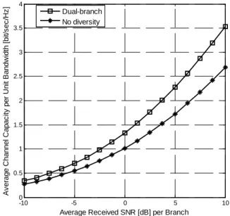
OPRA

η has been truncated at the 15th for drawing fig. 1. In fig. 1, the average channel capacity per unit bandwidth of dual-branch SC under OPRA scheme is plotted as a function of the average received SNR per branchγ . For comparison, the average channel capacity per unit bandwidth of Nakagami-0.5 fading channel without diversity, which was obtained in [12, Eq. (8)], is also presented in fig. 1. As expected, by increasing γ and/or employing diversity,

average channel capacity per unit bandwidth improves.

-10 -5 0 5 10

0 0.5 1 1.5 2 2.5 3 3.5 4

Average Received SNR [dB] per Branch

A

v

e

ra

g

e

C

h

a

n

e

l

C

a

p

a

c

it

y

p

e

r

U

n

it

B

a

n

d

w

id

th

[

b

it/

s

e

c

/H

z

]

Dual-branch No diversity

Figure 1. Average channel capacity per unit bandwidth

under OPRA for a Nakagami-0.5 fading channels versus average received SNR.

Table 2. shows P_OPRA_,_N at two different levels of truncation, N=5 andN=15, for dual-branch SC along with its truncation error bounds

up E OPRA P

−

, , andPOPRA, _E₋_low.

Table 2. Comparison ofP_OPRA_,_N,

up E OPRA

P _, ₋ ,and

low E OPRA P

−

, at two different values of N for worst case of fading.

5

= N

[ ]

dB

γ ηN_OPRA ηE−upOPRA ηE−lowOPRA

-10 0.1844003 0.35140 0.14825

-5 0.5073238 0.28697 0.18892

0 1.0859664 0.26870 0.23936

5 1.9739237 0.31500 0.30073

10 3.1482559 0.38678 0.37233

15

= N

[ ]

dB

γ ηN_OPRA ηE−upOPRA ηE−lowOPRA

-10 0.2534597 0.16563 0.08559

-5 0.6017111 0.14023 0.10093

0 1.2117708 0.13305 0.11996

5 2.1379537 0.14709 0.14311

10 3.3568817 0.17511 0.17011

5

= N

[ ]

dB

γ POPRA,N POPRA, _E₋_up POPRA, _E₋_low

-10 0.6232582539 0.0653675 1.5667192×10-4

-5 0.4383344079 0.0474504 8.3288090×10-6

0 0.2584629245 0.0287698 1.8807318×10-7

5 0.1253386000 0.0142201 1.6584278×10-9

10 0.0509878788 0.0058436 6.169986×10-12

15

= N

[ ]

dB

γ POPRA,N POPRA,_E₋_up POPRA,_E₋_low

-10 0.6232599015 0.0257515 0

-5 0.4383344613 0.0186926 0

0 0.2584629251 0.0113360 0

5 0.1253386000 0.0056019 0

(8)

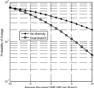
It is seen in table that the truncation error bounds become tighter as the truncation level,N , increases. Hence in order to get desired accuracy the infinite series in P_OPRA has been truncated at the 15th for drawing fig. 2.

In fig. 2, the probability of outage of dual-branch SC under OPRA scheme is plotted as a function of the average received SNR per branchγ . For comparison, the probability of outage of Nakagami-0.5 fading channel without diversity, which was obtained in [12, Eq. (9)], is also presented in fig.2. As expected, by increasing γ and/or employing diversity, probability of outage improves

-10 -5 0 5 10

10-2 10-1 100

P

ro

b

a

b

ili

ty

o

f

O

u

ta

g

e

No diversity Dual-branch

Figure 2. Probability of outage for a Nakagami-0.5 fading

channels versus average received SNR under OPRA scheme.

In fig. 3, the average channel capacity per unit bandwidth of dual-branch SC under TIFR scheme is plotted as a function of the cutoff SNR

γ

₀ for several values of the average received SNR per branchγ . As expected, by increasing γ average channel capacity per unit bandwidth improves.

-100 -5 0 5 10

0.5 1 1.5 2 2.5 3 3.5

Cutoff SNR [ dB]

A

v

e

ra

g

e

C

h

a

n

e

l

C

a

p

a

c

it

y

p

e

r

U

n

it

B

a

n

d

w

id

th

[

b

it/

s

e

c

/H

z

]

Average Received SNR per Branch= -10 dB Average Received SNR per Branch= -5 dB Average Received SNR per Branch= 0 dB Average Received SNR per Branch= 5 dB Average Received SNR per Branch= 10 dB

Figure 3. Average channel capacity per unit bandwidth for a

Nakagami-0.5 fading channels with dual-branch SC versus the cutoff SNR under TIFR scheme.

Table 3. shows P_TIFR_,_N at two different levels of truncation, N=45 andN=55, for dual-branch SC along with its truncation error bounds

up E TIFR

P , ₋ , and

low E TIFR

P , ₋ . It is seen in table that the truncation error

bounds become tighter as the truncation level, N , increases.

Table 3. Comparison of P_TIFR_,_N,

up E TIFR

P _, ₋ ,and

low E TIFR

P _, ₋ at two different values of N for worst case of fading.

Hence in order to get desired accuracy the infinite series in

TIFR

P has been truncated at the 55 th for drawing fig. 4.

-10 -5 0 5 10

10-2 10-1 100

P

ro

b

a

b

ili

ty

o

f

O

u

ta

g

e

No diversity Dual-branch

channels versus average received SNR under TIFR scheme.

45

= N

[ ]

dB

γ PTIFR,N PTIFR,_E₋_up PTIFR,_E₋_low

-10 0.767417818 0.0108675 0

-5 0.634092244 0.00918851 0

0 0.472983905 0.00702055 0

5 0.338303036 0.00509988 0

10 0.231889515 0.0035177 0

55

= N

[ ]

dB

γ PTIFR,N PTIFR,_E₋_up PTIFR,_E₋_low

-10 0.766182507 0.00894409 0

-5 0.632856933 0.00756222 0

0 0.471748594 0.0057797 0

5 0.337067725 0.00419725 0

(9)

In fig. 4, using the cutoff SNR levelsγ₀, the probability of outage with dual-branch SC under TIFR scheme is plotted as a function of the average received SNR per branchγ . For comparison, the probability of outage of uncorrelated Nakagami-0.5 fading channels with dual-branch SC and without diversity, which was obtained in [12], is also presented in fig. 4. As expected, by increasing γ and/or employing diversity, probability of outage improves.

Table 4. showsP

[

γ≥γ₀

]

_N, at two different levels of truncation, N=45 and N=55, for dual-branch SC along with its truncation error bounds P

[

γ≥γ₀

]

_upper and

[

]

lower

Pγ≥γ₀ .

Table 4. Comparison ofP

[

γ ≥γ₀

]

_N, P

[

γ ≥γ₀

]

_upper and

[

]

lower

Pγ ≥γ₀ at two different values of N for worst case of fading.

It is seen that the truncation error bounds becomes tighter as the truncation level N increases. Note that the truncation levels that were used to calculate the average channel capacity for table 5 isN=55.

Table. 5. shows TIFR

N

η at two different levels of truncation, 45

=

N andN = 55 , for dual-branch SC along with its truncation error bounds

TIFR

up E−

η and

TIFR

low

E−

η . It is seen that the truncation error bounds becomes tighter as the truncation level N increases. Hence in order to get desired accuracy the infinite series in

η

_TIFR has been truncated at the 55th for drawing fig. 5.

Table 5. Comparison of

TIFR

N

η ,

TIFR

up E−

η , and

TIFR

low

E−

η at two different values of N for worst case of fading

Figure.5 depicts the average channel capacity per unit bandwidth of a dual-branch SC system over uncorrelated Nakagami-0.5 fading channels under TIFR scheme as a function of the average received SNR per branchγ . For comparison, the average channel capacity per unit bandwidth of Nakagami-0.5 fading channel without diversity, which was obtained in [12, Eq.(18)], is also presented in fig. 5.

-100 -5 0 5 10

0.5 1 1.5 2 2.5 3 3.5

A

v

e

ra

g

e

C

h

a

n

e

l

C

a

p

a

c

it

y

p

e

r

U

n

it

B

a

n

d

w

id

th

[

b

it/

s

e

c

/H

z

]

Dual-branch No diversity

Figure 5. Average channel capacity per unit bandwidth

under TIFR for a Nakagami-0.5 fading channels versus average received SNR.

45

= N

[ ]

dB

γ P

[

γ≥γ₀

]

_N P

[

γ≥γ₀

]

_upper P

[

γ≥γ₀

]

_lower

-10 0.232582182 0.0833333 0.00691896

-5 0.365907756 0.0833333 0.00691896

0 0.527016095 0.0833333 0.00691896

5 0.661696963 0.0833333 0.00691896

10 0.768110485 0.0833333 0.00691896

55

= N

[ ]

dB

γ P

[

γ ≥γ₀

]

_N P

[

γ≥γ₀

]

_upper P

[

γ ≥γ₀

]

_lower

-10 0.23381749 0.0666667 0.00568365

-5 0.36714307 0.0666667 0.00568365

0 0.52825140 0.0666667 0.00568365

5 0.66293227 0.0666667 0.00568365

10 0.76934579 0.0666667 0.00568365

45

= N

[ ]

dB

γ ηN_TIFR ηE−upTIFR ηE−lowTIFR

-10 0.30454776 0.109118289 9.0598×10-3

-5 0.629511362 0.143367442 0.01190345

0 1.18533825 0.187429091 0.01556178

5 2.016898662 0.254005731 0.02108947

10 3.108404873 0.337234865 0.02799979

55

= N

[ ]

dB

γ ηN_TIFR ηE−upTIFR ηE−lowTIFR

-10 0.306165297 0.0872947 7.442285×10-3

-5 0.631636609 0.1146940 9.778208×10-3 0 1.188116636 0.1499434 0.012783381

5 2.020663964 0.2032048 0.017324163

(10)

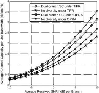
As expected, by increasing γ and/or employing diversity, average channel capacity per unit bandwidth improves. In fig. 6, the average channel capacity per unit bandwidth of uncorrelated Nakagami-0.5 fading channels is plotted as a function of γ , considering OPRA, and TIFR adaptation schemes with the aid of (27), and (35). It shows that, for Nakagami-0.5 fading channel condition OPRA achieves the highest capacity, whereas TIFR achieves the lowest capacity. As expected by increasing γ the channel capacity difference between OPRA and TIFR adaptation scheme increases slightly more in dual-branch SC since probability of outage improves.

-10 -5 0 5 10

0 0.5 1 1.5 2 2.5 3 3.5 4

Average Received SNR [ dB] per Branch

A

v

e

ra

g

e

C

h

a

n

e

l

C

a

p

a

c

it

y

p

e

r

U

n

it

B

a

n

d

w

id

th

[

b

it/

s

e

c

/H

z

]

Dual-branch SC under TIFR No diversity under TIFR Dual-branch SC under OPRA No diversity under OPRA

Figure 6. Average channel capacity per unit bandwidth for a

Nakagami-0.5 fading channel versus average received SNR

γ

using different adaptation scheme.

In fig. 7, it is depicted that for the Nakagami-0.5 fading conditions, OPRA achieves improved probability of outage compared to TIFR.

-10 -5 0 5 10

10-2 10-1 100

P

ro

b

a

b

ili

ty

o

f

O

u

ta

g

e

No diversity under OPRA Dual-branch SC under OPRA No diversity under TIFR Dual-branch SC under TIFR

channels versus average received SNR under different adaptation schemes.

It can also be observed that the probability of outage of TIFR for dual-branch SC is higher than the probability of outage OPRA with no diversity using [12].

5. Conclusions

In this paper, we analyze the average channel capacity and probability of outage of dual-branch SC over uncorrelated Nakagami-0.5 fading channels for OPRA and TIFR schemes. Closed-form expressions for the average channel capacity and probability of outage of dual-branch SC for OPRA and TIFR schemes have been obtained. Numerically evaluated results have been plotted and compared. It has been found that by increasing γ and/or employing diversity, average channel capacity improves for both the cases OPRA and TIFR. But the amount of improvement is slightly larger in case of OPRA. The probability of outage with dual-branch SC under TIFR is higher than the probability of outage with no diversity using OPRA, even when average received SNR

γ increases. It is very important to note that probability of outage under TIFR scheme is not improved adequately than the probability of outage under OPRA even as dual-branch SC is applied. This paper finally conclude that Nakagami-0.5 fading channels using TIFR scheme remains in outage for longer duration than using OPRA, even employing diversity and / or increasing average received SNRγ .

References

[1] A. Iqbal, A.M. Kazi, "Integrated Satellite-Terrestrial System Capacity Over Mix Shadowed Rician and Nakagami Channels," International Journal of Communication Networks and Information Security (IJCNIS), Vol. 5, No. 2, pp. 104-109, 2013.

[2] R.Saadane, M. Wahbi, “UWB Indoor Radio Propagation Modelling in Presence of Human Body Shadowing Using Ray Tracing Technique,’' International Journal of Communication Networks and Information Security (IJCNIS) Vol. 4, No. 2, 2012.

[3] S. Khatalin, J.P.Fonseka, “Channel capacity of dual-branch diversity systems over correlated Nakagami-m fading with channel inversion and fixed rate transmission scheme,” IET Communications, Vol. 1, No.6, pp.1161-1169, 2007.

[4] S.Khatalin, J.P.Fonseka, “Capacity of Correlated Nakagami-m Fading Channels With Diversity Combining Techniques,” IEEE Transactions on Vehicular Technology.,” Vol. 55, No.1, pp.142-150, 2006.

[5] V. Hentinen, “Error performance for adaptive transmission on fading channels,” IEEE Transactions on Communications, Vol. 22, No. 9, pp. 1331-1337, 1974.

[6] A. J. Goldsmith, P. P. Varaiya, “Capacity of Fading Channels with Channel Side Information,” IEEE Transactions on Information Theory,” Vol. 43, No. 6, pp. 1986-1992, 1997. [7] M. S. Alouini, A. Goldsmith, “Capacity of Nakagami

multipath fading channels,” Proceedings of the IEEE Vehicular Technology Conference., Phoenix, AZ, pp. 358-362, 1997.

[8] M. S. Alouini, A.J. Goldsmith, “Capacity of Rayleigh Fading Channels Under Different Adaptive Transmission and Diversity-Combining Techniques,” IEEE Transactions on Vehicular Technology, Vol. 48, No. 4, pp.1165-1181, 1999. [9] M .S. Alouini, A. Goldsmith, “Adaptive Modulation over

Nakagami Fading channels,” Wireless Personal Communication, Vol. 13, pp. 119-143, 2000.

(11)

[11] P.S.Bithas, P.T.Mathiopoulos, “Capacity of Correlated Generalized Gamma Fading With Dual-Branch Selection Diversity,” IEEE Transactions on Vehicular Technology, Vol. 58, No. 9, pp.5258-5263, 2009.

[12] M.I.Hasan, S.Kumar, “Channel Capacity of Dual-Branch Maximal Ratio Combining under worst case of fading scenario,” WSEAS Transactions on Communications, Vol. 13, pp. 162-170, 2014.

[13] S. Khatalin, J.P.Fonseka, “On the Channel Capacity in Rician and Hoyt Fading Environments With MRC Diversity,” IEEE Transactions on Vehicular Technology, Vol.55, No.1, pp.137-141, 2006.

[14] D.Brennan, “Linear Diversity Combining techniques,” Proceedings of IEEE, Vol.91, No.2, pp.331-354. 2003. [15] M. K. Simon, M. S. Alouini, Digital Communication over

Fading Channels, 2nd ed., New York: Wiley, 2005.

[16] G. Fodele, I.Izzo, M. Tanda, “Dual diversity reception of M-ary DPSK signals over Nakagami fading channels,” In Proceedings of the IEEE International Symposium Personal, Indoor, and Mobile Radio Communications, Toronto, Ont., Canada, pp.1195-1201, 1995.

[17] I. S. Gradshteyn, I. M. Ryzhik, Table of Integrals, series, and products, 6th ed., New York: Academic Press, 2000.