Semiparametric
regression
analysis
for
composite
endpoints
subject
to
componentwise
censoring
BY GUOQINGDIAO
DepartmentofStatistics,GeorgeMasonUniversity,4400UniversityDrive, Fairfax,Virginia22030,U.S.A.
DONGLINZENG
DepartmentofBiostatistics,CB7420,UniversityofNorthCarolina,ChapelHill, NorthCarolina27599,U.S.A.
CHUNLEIKE,HAIJUNMA,QIJIANG
AmgenInc.,OneAmgenCenterDrive,ThousandOaks,California91320,U.S.A. [email protected] [email protected] [email protected]
AND JOSEPHG.IBRAHIM
DepartmentofBiostatistics,CB7420,UniversityofNorthCarolina,ChapelHill, NorthCarolina27599,U.S.A.
SUMMARY
Composite endpointswith censored data arecommonly used asstudyoutcomesin clinical trials.Forexample,progression-freesurvivalisawidelyusedcompositeendpoint,withdisease progressionanddeathasthetwocomponents.Progression-freesurvivaltimeisoftendefinedas thetimefromrandomizationtotheearlieroccurrenceofdiseaseprogressionordeathfromany cause.Thecensoringtimesofthetwocomponentscouldbedifferentforpatientsnotexperiencing theendpointevent.Conventionalapproaches,suchastakingtheminimumofthecensoringtimes ofthetwocomponentsasthecensoringtimeforprogression-freesurvivaltime,maysufferfrom efficiency lossandcouldproduce biasedestimates ofthe treatment effect.Weproposea new likelihood-basedapproachthatdecomposestheendpointsandmodelsboththeprogression-free survivaltimeandthetimefromdiseaseprogressiontodeath.Thecensoringtimesfordifferent components aredistinguished.Theapproach makesfulluseofavailableinformationand pro-videsadirect andimprovedestimateofthetreatmenteffecton progression-freesurvivaltime. Simulationsdemonstratethattheproposedmethodoutperformsseveralotherapproachesandis robustagainstvariousmodelmisspecifications.Anapplicationtoaprostatecancerclinicaltrial isprovided.
1. INTRODUCTION
Composite endpoints, which consist of multiple component endpoints, are commonly used in clinical trials. Experiencing any of the events specified by the components is considered experiencing the composite endpoint. In particular, in oncology trials, progression-free survival is a composite endpoint with disease progression and death as the two components, and is defined as the time from randomization to the occurrence of disease progression or death from any cause. One example is the bone metastasis-free survival, with bone metastasis progression and death being the two components. Other examples of composite endpoints include cardiovascular death or hospitalization for heart failure, and major adverse cardiac events.
The censoring times for the individual components of a composite endpoint may not be the same. Using progression-free survival as an example, the two components, disease progression status and survival status, are often assessed using different schedules and methods, and are potentially subject to different censoring mechanisms, so the censoring times of the two com-ponents could differ for patients not experiencing the endpoint event. For example, assessment of objective disease progression requires radiological imaging evaluations. The progression-free status can only be confirmed up to the last evaluation, while the survival status can be assessed more frequently and thus confirmed up to a later time-point. Componentwise censoring can also occur when we retrieve information about survival status from public records for subjects who withdraw from clinical trials; for example, see the U.S. Food and Drug Administration’s guidance document on data retention (FDA,2008). However, not all death records are retrievable. When these events are included in a progression-free survival analysis, it is not clear how the censoring time should be defined for early-withdrawal subjects.
Componentwise censoring poses major challenges in the analysis of composite endpoints. Some conventional approaches include taking the minimum or the maximum of the censoring times of the two components. For example, in the U.S. Food and Drug Administration’s guidance document on oncology clinical trials (FDA,2007), it is recommended to censor progression-free survival time at the last assessment that determined a lack of progression. Death after two or more missed visits should be censored at the last assessment date before the missed visits. In practice, other methods may be used, such as censoring at the maximum censoring time for all component events, or treating withdrawal or change of therapy prior to disease progression as events (EMA,2008). However, these methods either do not take advantage of the full information on all components, or impose assumptions that are hard to verify. As a result, conventional approaches may suffer from efficiency loss and could produce biased parameter estimates.
In a 2015 unpublished paper, Y. Y Chen, C. Ke and J. Wang addressed different censoring schemes for component events through imputation. They proposed three multiple imputation-based methods: imputing the event time marginally using Kaplan–Meier estimates; imputing based on a Cox proportional hazards model; and imputing the event time of one component event based on a Kaplan–Meier estimate conditional on the other event. The risk set for sampling may become small towards the tail, leading to large variation. Furthermore, the inference procedure relies on simulation and can be computationally intensive. Boruvka & Cook(2016) developed sieve estimation in a Markov illness-death process under componentwise censoring, using a Cox-type proportional intensity model for each possible transition and assuming the baseline cumulative intensity functions to have piecewise parametric forms.
In this article, we develop a new likelihood-based approach to handle different censoring times for the individual components in a composite endpoint. The proposed model decomposes the endpoints and models both the progression-free survival time and the time from disease progression to death. The likelihood is derived, and the parameters including the treatment effect on progression-free survival time are estimated by maximizing the likelihood. The censoring times for different components are distinct and linked to individual components. Therefore, this approach makes full use of the available information and improves the estimate of the treatment effect on progression-free survival time. Furthermore, the proposed method provides insights into the covariate effects on the time from disease progression to death among patients who experience disease progression before death.
2. MODELS
Let Ts denote the time from randomization to disease progression and Td the time from randomization to death. The composite endpoint progression-free survival time is defined as Y =min(Ts,Td), i.e., the time to the first occurrence of disease progression or death. Our main interest is to study the treatment effect on this composite endpoint in the presence of right-censored data. We propose to model Y given X directly, which includes both treatment and baseline covariates, via the proportional hazards model
λ(t|X)=λ(t)exp(XTβ), (1)
whereλ(t)is the baseline hazard function andβrepresents the effect ofX on the log hazard rate ofY. Model (1) explicitly gives treatment effects on composite endpoint and survival profiles. We propose to model the baseline cumulative hazard(t)=0tλ(s)dsparametrically. For example, we assume that(t)=(t/α)θ, which corresponds to a Weibull distribution. Hereafter we write (t;α,θ)andλ(t;α,θ)to emphasize that the baseline cumulative hazard and baseline hazard functions forY depend on parametersαandθ.
Since death is always the end observation for any subject, our second model will involve the conditional distribution ofG≡Td −Y givenX andY; that is, we model the distribution of the time from the occurrence of the composite event to death. Clearly, if a patient never experiences disease progression,Td will be the same as Y; otherwise,Y = Ts is strictly less thanTd. This implies thatGhas a positive probability of being degenerate at zero. Therefore, we propose to modelGgivenX andY using a zero-inflated hazard model
where q(X,Y;ξ) = pr(G = 0 | X,Y;ξ)andA(t)is the baseline cumulative hazard function for G in the subpopulation where G > 0. Although we assume a parametric form forλ(t)in model (1), we leaveA(t)in (2) fully nonparametric, since we are interested in a model forY but are willing to leave the model forGas nonparametric as possible. We modelq(X,Y;ξ)by the logistic regression model
q(X,Y;ξ)= exp{ξ0+(X,Y) Tξ
1}
1+exp{ξ0+(X,Y)Tξ1}
, (3)
so the unknown parameters areψ ≡(η,A), whereη=(α,θ,β,ξ,γ )are the finite-dimensional parameters.
Define Cs and Cd to be the censoring times for Ts andTd, respectively. Typically a study design ensures thatCs Cd. Therefore, the observed data containO ≡ { ˜Y,Z˜,1,2,3,X},
where Y˜ = min(Ts,Td,Cs), Z˜ = min(Td,Cd), 1 = I(Ts CsandTs < Td), 2 =
I(Y˜ = Td) and 3 = I(Td Cd), with I(·) denoting the indicator function. Define fY(t | X;α,θ,β) = λ(t;α,θ)exp(XTβ)exp{−(t;α,θ)exp(XTβ)} and SY(t | X;α,θ,β) = exp{−(t;α,θ)exp(XTβ)}to be the density function and survival function ofY givenX, respec-tively. Additionally, define fG(t | X,t1;A,γ ) = a(t)exp{(X,t1)Tγ}exp[−A(t)exp{(X,t1)Tγ}]
andSG(t |X,t1;A,γ )=exp[−A(t)exp{(X,t1)Tγ}]to be respectively the density function and
survival function ofGgivenY =t1andX in the subpopulation whereG >0. Herea(·)is the
first derivative ofA(·).
Assume conditional independent censoring, i.e., that the censoring times (Cs,Cd) are inde-pendent of (Ts,Td)givenX. We next derive the likelihood contribution from a random sample Ounder five possible scenarios, (a)–(e).
Scenario (a): 1 = 3 = 1. Both Y = ˜Y and G = ˜Z − ˜Y are observed. Therefore the
likelihood contribution isW1(O;ψ)=fY(Y˜ |X;α,θ,β){1−q(X,Y˜;ξ)}fG(Z˜− ˜Y |X,Y˜;A,γ ). Scenario (b):2 = 3 = 1. We observe death at Y˜ = ˜Z, but no disease progression was
observed before Y˜. ThereforeY = ˜Y andG = 0. The likelihood contribution isW2(O;ψ) =
q(X,Y˜;ξ)fY(Y˜ |X;α,θ,β).
Scenario (c):1 =2=0 and3 =1. The patient was observed to stop disease progression
assessment or to drop out atY˜ without disease progression, but later died atZ˜. ThereforeY = ˜Z with probability q(X,Z˜;ξ) and Y ∈ (Y˜,Z˜) with probability 1−q(X,Y˜;ξ). The likelihood contribution is
W3(O;ψ)=q(X,Z˜;ξ)fY(Z˜ |X;α,θ,β)
+
Z˜−
˜ Y
fY(t|X;α,θ,β){1−q(X,t;ξ)}fG(Z˜ −t|X,t;A,γ )dt.
Scenario (d):1=1 and3=0. We observeY = ˜YbutGis censored atZ˜− ˜Y. The likelihood
contribution isW4(O;ψ)= {1−q(X,Y˜;ξ)}fY(Y˜ |X;α,θ,β)SG(Z˜ − ˜Y |X,Y˜;A,γ ).
Scenario (e):1 = 2 = 3 = 0. In this case,Y˜ = Cs,Z˜ = Cd, and bothY andTd are censored. The likelihood contribution is
W5(O;ψ)=
∞
˜ Z
q(X,t;ξ)fY(t|X;α,θ,β)dt
+
∞
˜ Z
t2
˜ Y
where the first term corresponds to the case where Y = Td andG = 0, and the second term corresponds to the case whereY =TsandG>0. One can show that
W5(O;ψ)=SY(Z˜ |X;α,θ,β)
+
Z˜
˜ Y
{1−q(X,s1;ξ)}fY(s1|X;α,θ,β)SG(Z˜ −s1 |X,s1;A,γ )ds1.
DefineI1(O) = I(1 = 3 = 1),I2(O) = I(2 = 3 = 1), I3(O) = I(1 = 2 = 0,
3 = 1), I4(O) = I(1 = 1,3 = 0) and I5(O) = I(1 = 2 = 3 = 0). The
like-lihood function of ψ based on n independent observations {Oi ≡ (Y˜i,Z˜i,1i,2i,3i,Xi)} (i = 1,. . .,n)isLn(ψ) = ni=1j=5 1Wj(Oi;ψ)Ij(Oi). Naturally, one would maximize Ln(ψ) to obtain an estimator of ψ. However, for a function A with fixed values at the observed gap times, we can always leta(Z˜i− ˜Yi)go to∞for subjectiwithI1(Oi) =1. Therefore, we apply
nonparametric maximum likelihood estimation by letting the estimator be a step function with jumps at the observed values forG. Suppose that 0< τ1<· · ·< τmare themdistinct observed
gap timesG. Using the nonparametric likelihood approach,A(t)=j:τjtA{τj}, whereA{t}is the jump size ofA(·)att. For ease of notation, we denote the resulting nonparametric likelihood function byLn(ψ)and the corresponding nonparametric loglikelihood byln(ψ).
We show how to calculate the integrals inW3(O;ψ)andW5(O;ψ)by using nonparametric
maximum likelihood. Under scenario (c), the second term of the likelihood contribution based on an observationOis
j:τj<Z˜− ˜Y
{1−q(X,Z˜ −τj,X;ξ)}A{τj}
×exp (X,Z˜ −τj)Tγexp−A(τj)exp{(X,Z˜ −τj)Tγ} ×λ(Z˜ −τj;α,θ)exp(XTβ)exp −(Z˜ −τj;α,θ)exp(XTβ).
We now turn our attention to scenario (e). Defineτm+1 = ∞and 0= g0 <g1 < · · ·< gk gk+1 = ˜Z − ˜Y < τk+1, wheregj =τj (j=1,. . .,k). We can show that the second term of the likelihood contribution inW5(O;ψ)can be written as
Z˜
˜ Y {
1−q(X,s1;ξ)}fY(s1|X;α,θ,β)SG(Z˜ −s1 |X,s1;A,γ )ds1
=
k
j=0
Z˜−gj
˜ Z−gj+1
{1−q(s1,X;ξ)}fY(s1 |X;α,θ,β)SG(τj |X,s1;A,γ )ds1.
We use Gauss–Legendre quadrature to approximate the above integrals. In our experience, the Gauss–Legendre quadrature is reasonably accurate with ten abscissa points. To maximizeLn(ψ), we use the quasi-Newton algorithm (Press et al.,1992). The resulting nonparametric maximum likelihood estimators ofψ are denoted byψnˆ ≡(ηnˆ ,Aˆn).
3. ASYMPTOTIC PROPERTIES
Assumption1. The covariate X has bounded support. IfcT
1X = c0 with probability 1, then
c0=0 andc1 =0.
Assumption2. There exists some positive constantδ1 such that pr(Cs τ | X) = pr(Cs = τ |X)δ1almost surely, whereτ is a constant denoting the end of the study. Additionally, with
probability 1,CsCd.
Assumption3. The true parameter values of(α,θ,β,ξ,γ ), denoted byη0 ≡(α0,θ0,β0,ξ0,γ0),
lie in the interior of a known compact set in the domain ofη.
Assumption 4. The true baseline cumulative hazard function A0 is strictly increasing and
continuously differentiable in[0,τ].
Assumption1is the usual condition for a design matrix in regression settings to ensure model identifiability. Assumptions3and4and the first part of Assumption2are standard regularity and technical conditions for a regression model with right-censored data. Assumption2also implies pr(Cd τ |X)=pr(Cd =τ |X)δ1. Assumptions1and4imply that pr(Td >Ts |X)δ2
for some positive constantδ2; hence some patients experience disease progression before death
and so we can observe the gap timeGwith a positive probability.
We show in theSupplementary Materialthat the unknown parametersηandA(t) (t ∈ [0,τ]) are identifiable. We next establish consistency and asymptotic normality of the proposed nonparametric maximum likelihood estimators in the following two theorems.
THEOREM1. Under the conditional independent censoring assumption and Assumptions1–4, with probability tending to 1, ˆηn −η0 +supt∈[0,τ]| ˆAn(t)−A0(t)| → 0, where · is the
Euclidean norm.
THEOREM2. Under the conditional independent censoring assumption and Assumptions1–4, n1/2(ηnˆ −η0,Aˆn −A0) → G in distribution, where G is a continuous zero-mean Gaussian
process in l∞(H) and H = {(h1,h2) : h1 ∈ R3p+5,h2(·)is a function on[0,τ];h1 1,
|h2(t)|V[0,τ] 1}. Here l∞(H)denotes the space of all bounded linear functionals onHand
|h|V[0,τ]denotes the total variation of h in[0,τ]. Furthermore, the limiting covariance matrix of
n1/2(ηnˆ −η0)attains the semiparametric efficiency bound.
Theorem1states the consistency of the nonparametric maximum likelihood estimators. The basic idea in the proof of Theorem 1is as follows. We first show by contradiction that Aˆn(τ) cannot diverge. Once the boundedness ofAˆn(τ)is established, a subsequence ofAˆncan be found that converges pointwise to a bounded monotone functionA∗in[0,τ], and the same sequence of ηnˆ converges to someη∗. We construct a step function A¯n with jumps at the observed gap times converging to A0. Finally, we prove that the Kullback–Leibler information between the
true density and the density indexed by (η∗,A∗)is nonpositive. Consistency will then follow from the identifiability result. The details are given in the Appendix.
Theorem 2 implies that for any (h1,h2) ∈ R3p+5 × l∞(H), n1/2(ηnˆ − η0)Th1 +
n1/20τ h2(t)(dAˆn −dA0)is asymptotically normal with mean zero. This result can be derived
Table 1. Summary statistics for nonparametric maximum likelihood estimates based on 1000 replicateswithn=300
Parameter True Bias(×100) SE(×100) SEE(×100) CP(×100)
α 1 2·7 12·8 12·6 95
θ 1 1·7 6·4 6·5 94
β1 1 2·3 10·7 10·3 94
β2 −1 0·1 17·6 17·8 96
ξ0 0 6·7 30·5 29·1 94
ξ1 0·5 0·4 26·5 25·6 95
ξ2 0·5 7·3 54·0 49·6 95
γ1 1 −1·1 28·3 27·8 95
γ2 0·5 0·0 48·4 46·5 95
A(0·20) 0·2 0·9 8·7 8·5 96
A(0·25) 0·25 1·4 10·3 10·1 95
A(0·30) 0·3 1·9 12·0 11·6 94
A(0·35) 0·35 2·1 13·2 13·0 95
SE, sample standard deviation of the estimates; SEE, average of the standard error estimates; CP, coverage probability of the 95% confidence interval based on a normal approximation.
4. SIMULATION STUDIES
We conducted extensive simulation studies to examine the performance of the proposed non-parametric maximum likelihood estimators under joint modelling of the composite endpoint Y and the gap time G between Y and Td. We first generate two covariates, X1 ∼ N(0, 1) and
X2 ∼ Ber(1/2), and then generate the composite endpoint Y from the model (t | X) =
texp(β1X1 +β2X2). This implies that the true values of α and θ in the Weibull distribution
both equal 1. We next determine whether the composite endpoint isTsorTd based on a logistic regression model pr(G=0|X1,X2;ξ)=exp(ξ0+ξ1X1+ξ2X2)/{1+exp(ξ0+ξ1X1+ξ2X2)}.
If G = 0, then the composite endpoint is Td. Otherwise, we generateG based on the model A(t | X1,X2;γ ) = texp(γ1X1 +γ2X2). The true value of the cumulative hazard function for
G given G > 0 isA(t) = t. ThenTd = Ts+G. Finally, we generate the censoring time for Ts, denoted byCs, from an exponential distribution with mean 0·5; thenCd =Cs+u, whereu follows an exponential distribution with mean 2.
We set the true regression parameter values to be (β1,β2,ξ0,ξ1,ξ2,γ1,γ2) =
(1,−1, 0, 0·5, 0·5, 1, 0·5). The relative frequencies of the five scenarios (a)–(e) are 8·84%, 16·87%, 29·80%, 1·91% and 42·59%, respectively. We estimate the covariance matrix of (ηnˆ ,Aˆn) by inverting the observed Fisher information matrix, i.e., the negative second derivatives of the loglikelihood with respect toηand the jump sizes ofA(·), evaluated at(ηnˆ ,Aˆn). Table1shows that the estimators have low bias and that the standard errors reflect the actual variation of the estimates. The coverages of the 95% confidence intervals are close to the nominal level.
We also used four naive methods to analyse the composite endpoint. All treatY as the survival endpoint subject to right censoring. Denote the censoring time byCand the censoring indicator by = I(Y C). In scenarios (a), (b) and (d), we can directly observeY = ˜Y and therefore =1. In scenario (c) we do not observe the composite endpoint but we know thatY belongs to (Y˜,Z˜]. In scenario (e), the composite endpoint is censored but it is not clear whether the censoring time isY˜ orZ˜ or some other time-points betweenY˜ andZ˜. Table2provides the definitions of min(Y,C)andfor the naive methods in scenarios (c) and (e).
Table 2.Definitionofmin(Y,C)andforthefournaivemethods Naive method Scenario (c) Scenario (e)
(i) C= ˜Y,=0 C= ˜Y,=0 (ii) Y = ˜Z,=1 C= ˜Y,=0 (iii) C= ˜Y,=0 C= ˜Z,=0 (iv) Y = ˜Z,=1 C= ˜Z,=0
that time to death is the composite endpoint and ignore the possibility that disease progression occurs in the interval(Y˜,Z˜). In scenario (e), the censoring timeC ∈ [ ˜Y,Z˜]is unknown and is imputed with eitherY˜ orZ˜. FDA guidance recommends censoring patients without an event at the last adequate disease assessment date and to censor at the last disease assessment if death occurs after more than one missed disease assessment. This is similar to naive method (iii).
For all four methods, we fit the parametric Weibull proportional hazards model in order to have a fair comparison, since the true composite endpoint was generated from a Weibull distribution. We consider simulation settings similar to the above, but also incorporate Y in the model of pr(G=0|X1,X2,Y;ξ)andA(t|X1,X2,Y;γ ). The corresponding regression parameters forY
areξ3=γ3=0·5. Table3summarizes the results. The proposed method essentially outperforms
all naive methods in terms of mean squared error efficiency. Although the parameter estimates from naive method (i) have low biases, they are less efficient than the proposed estimators, because naive method (i) ignores the possibility that the composite endpoint is the observed death time under scenario (c). Naive method (ii) treats the observed death time as the composite endpoint under scenario (c) and therefore led to an excessive number of events. Consequently, the estimates from naive method (ii) have smaller variation but large biases. Similarly, naive method (iv) also yielded biased parameter estimates. Estimates from naive method (iii) have both large biases and large variations.
In the next set of simulation studies, we compared the performances of the Wald tests of the effect ofX2 based on the proposed method and the four naive methods. We consider the same
simulation setting as above except that β2 varies from 0 to −0·6. Table4 presents the Type I
error rates and powers at the 0·05 significance level based on 1000 replicates withn=300. The proposed method controls the Type I error rate accurately and is substantially more powerful than all four naive methods. In particular, naive methods (ii) and (iv) tend to have inflated Type I error rates.
Naive methods (ii) and (iv) replace the composite endpoint with the death time under scenario (c). Intuitively, the covariate effect on the composite endpoint is a complicated function of the covariate effects on both time to disease progression and time to death, as well as other parameters. Consequently, the covariate effect on the death time tends to contribute more to the covariate effect on the composite endpoint in naive methods (ii) and (iv). We consider a simple example to demonstrate this observation. Suppose thatTsandTd are independent. Then the hazard function for the composite endpoint is λ(t |X) =exp(βTX)+exp(γTX). Ifβ
1 = γ1, thenλ(t | X) =
exp(β1X1){exp(β2X2)+exp(γ2X2)}. The log hazard ratio of the composite endpoint for X2 is
then β2∗ =log[{exp(β2X2)+exp(γ2X2)}/2]. Therefore, it is possible that β2∗ =0 butβ2 |= 0
andγ2 |=0. For example, we letβ2 = 0·2 andγ2 = −0·25, yieldingβ2∗= 0. We conducted a
SD(×100)
Table 3. Comparison of the proposed method and four naive methods based on 1000 replicateswithn=300
Parameter Bias(×100) MSE(×100) RE
Proposed method
α 2·1 12·2 1·5
θ 2·1 6·6 0·5
β1 2·2 10·0 1·1
β2 0·4 17·4 3·0
Naive method (i)
α 1·5 17·8 3·2 2·10
θ 2·2 8·8 0·8 1·71
β1 2·3 13·1 1·8 1·66
β2 −1·3 23·7 5·7 1·87
Naive method (ii)
α −12·1 8·0 2·1 1·38
θ 12·6 6·6 2·0 4·20
β1 −11·6 9·2 2·2 2·09
β2 25·9 15·9 9·2 3·04
Naive method (iii)
α 112·8 48·4 150·7 99·04
θ −20·0 6·5 4·4 9·16
β1 19·0 13·1 5·3 5·03
β2 −15·1 23·9 8·0 2·63
Naive method (iv)
α 18·2 11·6 4·6 3·05
θ 1·6 6·3 0·4 0·87
β1 6·8 9·4 1·3 1·27
β2 9·5 15·6 3·3 1·10
SD, empirical standard deviation of the estimates; MSE, mean squared error; RE, mean squared error relative efficiency of the proposed estimators compared to the estimators using the naive methods.
Table 4.Type I error rate(×100)and power(×100)for testing the effect of X2on composite endpoints at significance level0·05based
on1000replicates with n=300
β2 Proposed Naive (i) Naive (ii) Naive (iii) Naive (iv)
0 5 5 6 5 8
−0·1 8 8 5 7 4
−0·2 23 18 11 18 12 −0·3 47 35 27 37 33
−0·4 71 50 45 54 56
−0·5 88 66 67 74 81
−0·6 96 80 83 88 94
Table 5. Frequenciesandrelativefrequencies ofthefivescenariosforthe prostatecancerdata
Standard treatment New treatment
Scenario Frequency Relative frequency (%) Frequency Relative frequency (%)
(a) 130 23·2 119 21·2
(b) 0 0·0 0 0·0
(c) 74 13·2 72 12·9
(d) 121 21·6 112 20·0
(e) 235 42·0 257 45·9
leading to interval-censored data. While the proposed method is not designed for such data, we impute the time to disease progression with the midpoint of the interval and then apply the proposed method, which seems to be reasonably robust in this situation. Details of these two sets of simulation studies are provided in theSupplementary Material.
5. APPLICATION
We now apply the proposed method to a randomized placebo-controlled clinical trial for non-metastatic prostate cancer patients at high risk for bone metastasis. The primary endpoint was bone metastasis-free survival, defined as time from randomization to bone metastasis or death, whichever occurs first. Events of bone metastasis were determined by central review of images collected periodically at baseline and on study, and therefore were censored at the last image assessment date for patients who did not experience an event. All-cause death was assessed via study contact, and was censored at the last study contact date for patients who were alive. Some patients discontinued image assessments but stayed on study for overall survival assessment, so they were censored earlier for bone metastasis but could die or be censored for death later. The study was stratified by previous or current use of chemotherapy and by high risk for metastasis based on prostate-specific antigen. The treatment phase of the study ended when a targeted number of patients developed bone metastasis or died. In addition, the study had a long-term survival follow-up phase, where patients who had progressed or who did not wish to continue the scheduled study assessment were followed for survival status only.
We analysed a randomly selected subset of 1120 patients provided by the trial sponsor, with 560 in each arm. The proposed method was used to analyse the composite endpoint of bone metastasis-free survival, adjusting for the stratification factors, and was compared with some naive methods and two existing methods. For the proposed method, three covariates were included in the model for the composite endpoint, the model for pr(G =0)and the model forGwhenG >0. These covariates are: trt, taking value 1 for new treatment and value 0 for standard treatment; chemo, taking value 1 for previous or current use of chemotherapy and value 0 otherwise; and psa, taking value 1 if the patient was assessed to be at high risk for metastasis based on prostate-specific antigen and value 0 otherwise. Among the 1120 patients, 80 had previous or current use of chemotherapy and 542 were at high risk based on prostate-specific antigen. We included Y in both the model for pr(G=0)and the model forGwhenG>0.
We used data in both the treatment and the long-term survival follow-up phases. Table 5
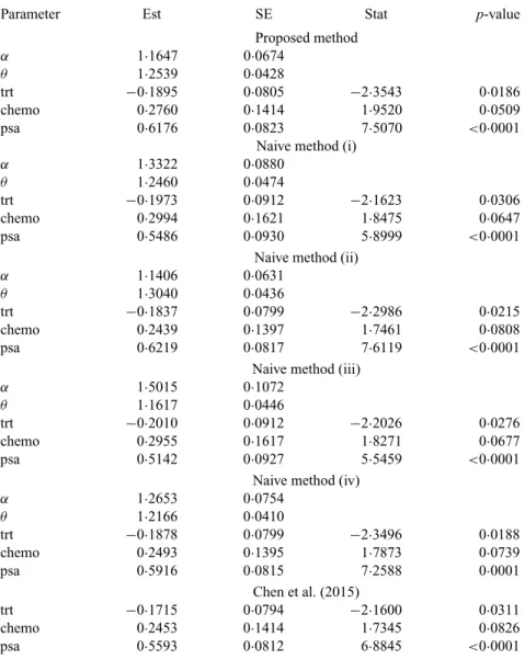
Table6. Resultsfromthemodelonbonemetastasis-freesurvivalforthe prostatecancerdata
Parameter Est SE Stat p-value
Proposed method
α 1·1647 0·0674
θ 1·2539 0·0428
trt −0·1895 0·0805 −2·3543 0·0186
chemo 0·2760 0·1414 1·9520 0·0509
psa 0·6176 0·0823 7·5070 <0·0001
Naive method (i)
α 1·3322 0·0880
θ 1·2460 0·0474
trt −0·1973 0·0912 −2·1623 0·0306
chemo 0·2994 0·1621 1·8475 0·0647
psa 0·5486 0·0930 5·8999 <0·0001 Naive method (ii)
α 1·1406 0·0631
θ 1·3040 0·0436
trt −0·1837 0·0799 −2·2986 0·0215
chemo 0·2439 0·1397 1·7461 0·0808
psa 0·6219 0·0817 7·6119 <0·0001
Naive method (iii)
α 1·5015 0·1072
θ 1·1617 0·0446
trt −0·2010 0·0912 −2·2026 0·0276
chemo 0·2955 0·1617 1·8271 0·0677
psa 0·5142 0·0927 5·5459 <0·0001 Naive method (iv)
α 1·2653 0·0754
θ 1·2166 0·0410
trt −0·1878 0·0799 −2·3496 0·0188
chemo 0·2493 0·1395 1·7873 0·0739
psa 0·5916 0·0815 7·2588 0·0001
Chen et al. (2015)
trt −0·1715 0·0794 −2·1600 0·0311
chemo 0·2453 0·1414 1·7345 0·0826
psa 0·5593 0·0812 6·8845 <0·0001
Est, parameter estimate; SE, standard error; Stat, Wald test statistic; trt, treatment indicator; psa, prostate-specific antigen.
With other covariates fixed, the odds that the composite endpoint is death for patients at high risk based on prostate-specific antigen was estimated at 1·939 times the odds for patients at low risk. The corresponding 95% confidence interval was (1·00, 3·76). We can draw similar conclusions from the results based on the proposed method and the method of Chen et al. However, there were notable differences in the parameter estimates, especially for the effect of psa. In addition, the inference procedure of Chen et al. requires simulation and thus is computationally more intensive.
6. DISCUSSION
Other parametric and semiparametric models may be used for the time to the composite endpoint and the gap time, respectively. The parametric assumption on the distribution of the composite endpoint may be relaxed through the use of B-splines over a sieve space. Furthermore, it would be desirable to develop diagnostic tools to check the goodness-of-fit of the proposed model. Future research along this direction is warranted.
In some applications, disease progression status is assessed periodically, leading to interval censoring.Zeng et al. (2015) showed that the right-endpoint imputation method would lead to biased estimation and reduced power when progression status is known only at periodic assess-ment times. While it is challenging to analyse interval-censored data by using semiparametric or nonparametric methods, we can extend the proposed models to this setting. Specifically, under models (1)–(3), we can derive the likelihood for each possible scenario of the observed data and develop inference procedures. This extension is currently under investigation. On the other hand, our simulation studies have demonstrated that the proposed method with midpoint imputation is reasonably robust with respect to interval censoring.
We considered a specific case where one component is terminal. In the case where no event terminates the other component event, one can choose one component event as the terminal event and apply the proposed approach. If one component event under monitoring is longer than the other component, the component event with the longer censoring time can be chosen as the terminal event. Otherwise, one can choose the lower-frequency component. Our method can also be extended without assuming this terminating structure.
Often a composite endpoint has more than two components. For example, in evaluating bone-target agents for advanced cancer patients, a composite endpoint of skeletal-related events includes four components: pathologic fracture, spinal cord compression, radiation to bone, and surgery to bone. In general, one can group components into two clusters and then apply the pro-posed method. For example, for the skeletal-related events, one group could consist of pathologic fracture, which is identified through regular skeletal survey, and the other three events could make up the second cluster, which is monitored through clinical visits.
ACKNOWLEDGEMENT
The authors are grateful to the referees and the associate editor for insightful comments.
SUPPLEMENTARY MATERIAL
Supplementary materialavailable atBiometrikaonline includes additional simulation studies,
the proof of identifiability of the proposed model, and further details of the proofs of Theorems1
and2.
APPENDIX
Proof of Theorem1
We introduce notation that will be used throughout the proofs of Theorems1and2. LetOi(i=1,. . .,n) denote the observations for theith subject. DefinePn{g(O)} =n−1
n
i=1g(Oi)andP{g(O)} =E{g(O)}. The proof of consistency consists of two main steps. In the first, we prove that lim supnAˆn(τ)has an upper bound with probability 1. Therefore, for any subsequence, there exists a further subsequence of
(ηˆn,Aˆn)that converges to(η∗,A∗)weakly by the Helly selection theorem. In the second step, we prove that (η∗,A∗)=(η
0,A0).
Step1. We prove the boundedness ofAˆn(τ)by contradiction. DefineRj(O;ψ) = logWj(O;ψ) (j =
1,. . ., 5), whereWj(O;ψ) (j=1,. . ., 5)are as defined in §2. Using the same notation for simplicity, we
replacea(t)withA{t}, the jump size ofA(·)att, inWj(O;ψ)andRj(O;ψ) (j=1,. . ., 5).
Defineνˆn = ˆAn(τ) andA˜n(t) = ˆAn(t)/ˆνn for t ∈ [0,τ]. To prove thatAˆnin[0,τ]is bounded, it is sufficient to show thatνˆnis bounded. By Assumptions1and3and the definition ofA˜n(t), we can show thatR1(O;ηˆn,Aˆn)−R1(O;ηˆn,A˜n)c1+logνˆn−c2A˜n(G˜)ˆνnfor some constantc1and a positive constant
c2. Furthermore, we can show thatR2(O;ηˆn,Aˆn)−R2(O;ηˆn,A˜n)=0,R3(O;ηˆn,Aˆn)−R3(O;ηˆn,A˜n)c3,
R4(O;ηˆn,Aˆn)−R4(O;ηˆn,A˜n)c3−c4A˜n(G˜)ˆνnandR5(O;ηˆn,Aˆn)−R5(O;ηˆn,A˜n)c3for some constant
c3and a positive constantc4.
Suppose thatνˆn→ ∞. It follows that, for some constantc5and a positive constantc6,
01
nln(ηˆn,Aˆn)− 1
nln(ˆηn,A˜n)
c5+logνˆn−c2Pn{I1(O)A˜n(G˜)}ˆνn−c4Pn{I4(O)A˜n(G˜)}ˆνn
c5+logνˆn−c6νˆn→ −∞,
where the penultimate inequality is obtained from the conditionally independent censoring assumption, Assumptions1,3and4, and the Glivenko–Cantelli theorem. This result contradicts the definition of(ηˆn,Aˆn). The above argument holds for every sample in the probability space except on a set with zero probability. Thus we have shown that, with probability 1,Aˆn(τ)is bounded for any sample of sizen. Therefore, by Helly’s selection theorem, we can choose a further subsequence, still indexed by{n}, such that(ˆηn,Aˆn) converges to(η∗,A∗)with probability 1.
Step 2. In this step, we show that (η∗,A∗) = (η0,A0). By differentiating ln(η,A) with respect to A{ ˜Gi}for1i=3i=1 and setting the derivative to zero, we can see thatAˆn{ ˜Gi}satisfies the equation
ˆ
An{ ˜Gi} =
I1(Oi)
nPn 5
k=1Ik(O)Qk(t,O;ηˆn,Aˆn)
t= ˜Gi
= I1(Oi)+nPnI3(O)Q31(t,O;ψˆn)
nPn
k∈{1,2,4,5}Ik(O)Qk(t,O;ψˆn)+I3(O)Q32(t,O;ψˆn)
t= ˜Gi ,
where the expressions for Qk(t,O;ψ) (k = 1,. . ., 5), Q31(t,O;ψ) andQ32(t,O;ψ) are given in the
Supplementary Material. We can easily verify that, with probability 1, Qk(t,O;ψˆn) (k = 1, 4, 5), Q31(t,O;ψˆn) and Q32(t,O;ψˆn) are nonnegative. Furthermore, for any G˜i with 1i = 3i = 1,
Pn{I1(O)Q1(G˜i,O;ψˆn)}is positive. Therefore, the denominator in (A1) is bounded away from zero, and for a subjectiwith1i=3i=1, Aˆn{ ˜Gi}is positive and bounded.
We next construct another step functionA¯n(t)with jumps only at the observed gap timeG˜iby replacing ˆ
ψnwithψ0in (A1). We verify thatA¯n(t)converges toA0uniformly int ∈ [0,τ]with probability 1. As
is shown in theSupplementary Material, the classF1 = {
5
k=1Ik(O)Qk(t,O;η,A):t ∈ [0,τ],η∈ B0,
A ∈ A,A(0)= 0}is bounded and P-Donsker, whereA = {g : gis a nondecreasing function in[0,τ], g(τ) B0}andB0is a positive constant such thatAˆn(τ) B0 with probability 1. Since a P-Donsker
class is also Glivenko–Cantelli, by the Glivenko–Cantelli theorem (van der Vaart & Wellner,1996),A¯n(t) converges uniformly toE{I1(O)/μ(t)}, whereμ(t)=E{
5
k=1Ik(O)Qk(t,O;η0,A0)}. By the conditional
independent censoring assumption, we can prove thatE{I1(O)/μ(t)} =A0(t). Consequently, we conclude
thatA¯nconverges uniformly toA0in[0,τ]with probability 1.
By the construction ofAˆn(t)andA¯n(t), we can see thatAˆn(t)is absolutely continuous with respect to ¯
An(t); furthermore, by letting ngo to infinity,A∗(t)is differentiable with respect toA0(t)so thatA∗(t)
is differentiable with respect tot. It follows that dAˆn(t)/dA¯n(t)converges to dA∗(t)/dA0(t)uniformly in
t∈ [0,τ].
By the definition of(ηˆn,Aˆn),n−1ln(ηˆn,Aˆn)−n−1ln(η0,A¯n)0. SinceB0×Ais a Donsker class and
the functionals Rk(O;η,A) (k = 1,. . ., 5)are bounded Lipschitz functionals with respect toB0×A,
the class F2 = {
5
k=1Ik(O)Rk(O;η,A) : η ∈ B0,A ∈ A,A(0) = 0, A(τ) B0} is P-Donsker
and hence a Glivenko–Cantelli class. Therefore, by taking n → ∞, the left-hand side in the above inequality converges to the negative Kullback–Leibler information. It then follows that, with probabil-ity 1,5k=1Ik(O)Rk(O;η∗,A∗)=
5
k=1Ik(O)Rk(O;η0,A0). Therefore, from the identifiability result, we
obtain(η∗,A∗)=(η0,A0). This completes the proof of Theorem1.
Proof of Theorem2
To prove Theorem2, we verify the four conditions (P1),. . ., (P4) in Theorem 3.3.1 ofvan der Vaart & Wellner(1996), which are listed in theSupplementary Material. We first define a neighbourhood of the true parameters(η0,A0)byU = {(η,A):η−η0 +supt∈[0,τ](|A(t)−A0(t)|) < 0}for a very small constant 0. Based on the consistency theorem,(ηˆn,Aˆn)belongs toU with probability close to 1 when the sample sizenis large enough.
For any one-dimensional submodel given as {η+h1,A+
h2dA} for (η,A) ∈ U and H ≡
(h1,h2)∈H, we can derive the score function for a single observationOasV(O;ψ)[H] =lη(O;ψ)Th1+
lA(O;ψ)[
h2dA], wherelη(O;ψ)=
5
k=1Ik(O)dRk(O;ψ)/dηand
lA(O;ψ)
h2dA
=I1(O)
h2(G˜)−exp{(X,Y˜)Tγ}
G˜
0
h2dA
+ I3(O)
exp{R3(O;ψ)}
G˜
0
{1−q(X,Z˜ −s,X;ξ)}exp{(X,Z˜ −s)Tγ}
×exp−A(s)exp{(X,Z˜ −s)Tγ}
h2(s)−exp{(X,Z˜−s)Tγ}
s
0
h2dA
×λ(Z˜ −s;α,θ)exp(XTβ)
exp−(Z˜ −s;α,θ)exp{XTβ} dA(s)
−I4(O)exp{(X,Y˜)Tγ}
G˜
0
− I5(O)
exp{R5(O;ψ)}
Z˜
˜ Y
{1−q(X,s1;ξ)}fY(s1|X;α,θ,β)
×SG(Z˜ −s1|X,s1;A,γ )exp{(X,s1)Tγ}
Z˜−s1
0
h2dAds1.
For ease of notation, we omit[H]fromV(O;ψ)[H]. We defineUn(ψ)=Pn{V(O;ψ)}andU(ψ)=
P{V(O;ψ)}. Thus it is easy to see that both Un(ψ) and U(ψ) are maps from U tol∞(H) and that n1/2{Un(ψ)−U(ψ)}is an empirical process in the spacel∞(H). It then follows thatUn(ψˆn) = 0 and U(ψ0)=0.
To prove property (P1), we make use of Lemma 3.3.5 ofvan der Vaart & Wellner(1996). Based on the explicit expression for the score function,V(O;η,A)[H]is continuously differentiable with respect toη anddV(O;η,A)/dηc9, wherec9is a positive constant. Furthermore,
V(O;η,A)−V(O;η,A˜)c10
I1(O)
|A(G˜)− ˜A(G˜)| + G
0
|A(t)− ˜A(t)|dt
+I3(O)
G˜
0
|A(s)− ˜A(s)|dA(s)+ G˜
0
|A(s)− ˜A(s)|dA˜(s)
+
G˜
0
|dA(s)−dA˜(s)|
+I4(O)|A(G˜)− ˜A(G˜)| +I5(O)
Z˜
˜ Y
|A(s)− ˜A(s)|ds
for some positive constant c10. Therefore supH∈HE[{V(O;η,A)−V(O;η,A)}2] converges to zero if
η−η0 +supt∈[0,τ]{|A(t)−A0(t)|} →0. Additionally, by using a similar argument to that in the proof of
Theorem1, we can show that the classF3= {V(O;η,A)[H] −V(O;η0,A0)[H]:(η,A)∈U,H ∈H}is
P-Donsker. Therefore, according to Lemma 3.3.5 ofvan der Vaart & Wellner(1996), property (P1) holds. Property (P2) holds because of the P-Donsker property of the class{V(O;η,A)[H]:H ∈H}. Further-more, the limit random elementsζ constitute a Gaussian process indexed byH ∈Hand the covariance betweenζ(H1)andζ(H2)is equal toE{V(O;η0,A0)[H1] ×V(O;η0,A0)[H2]}.
The Fréchet differentiability in (P3) can be directly verified using the smoothness of U(η,A). The derivative of U(η,A)at(η0,A0), denoted by U(η0,A0), is a map from the space {(η−η0,A−A0) : (η,A)∈U}tol∞(H).
It remains to show thatU is continuously invertible at(η0,A0). Following the argument in the appendix
ofZeng & Lin(2007), it suffices to prove that for any one-dimensional submodel given as{η+h1,A+ h2dA}forH ∈H, the Fisher information along this submodel is nonsingular. If the Fisher information
along this submodel is singular, the score function along this submodel is zero with probability 1. Using similar arguments to those in the proof of identifiability of the model, we can show thatV(O;η,A0)[H] =0
yieldsh1=0 andh2(t)=0 for anyt∈ [0,τ].
We now have verified properties (P1)–(P4), so Theorem 3.3.1 of van der Vaart & Wellner(1996) allows us to conclude thatn1/2(ˆηn−η0,Aˆn−A0)converges weakly to a tight Gaussian random element −U −1ζ inl∞(H). Moreover, it can be shown thatηˆ
nis an asymptotic linear estimator forη0and that the
corresponding influence functions are in the space spanned by the score functions. This implies thatηˆnis semiparametrically efficient by semiparametric efficiency theory.
REFERENCES
BORUVKA, A. & COOK, R. J. (2016). Sieve estimation in a Markov illness-death process under dual censoring. Biostatistics17, 350–63.
EMA (2008). Appendix 1 to the Guideline on the Evaluation of Anticancer Medicinal Products in Man
(chmp/ewp/205/95 rev. 3). London: European Medicines Agency.
FDA (2007). Guidance for Industry: Clinical Trial Endpoints for the Approval of Cancer Drugs and Biologics. Rockville, Maryland: U.S. Food and Drug Administration.
FDA (2008).Guidance for Sponsors, Clinical Investigators, and IRBs: Data Retention When Subjects Withdraw from FDA-Regulated Clinical Trials. Rockville, Maryland: U.S. Food and Drug Administration.
LI, Y. & ZHANG, Q. (2015). A Weibull multi-state model for the dependence of progression-free survival and overall
survival.Statist. Med.34, 2497–513.
PARNER, E. (1998). Asymptotic theory for the correlated gamma-frailty model.Ann. Statist.26, 183–214.
PRESS, W. H., TEUKOLSKY, S. A., VETTERLING, W. T. & FLANNERY, B. P. (1992).Numerical Recipes in C: The Art of Scientific Computing. Cambridge: Cambridge University Press, 2nd ed.
QUAN, H., ZHANG, D., ZHANG, J. & DEVLAMYNCK, L. (2007). Analysis of a binary composite endpoint with missing
data in components.Statist. Med.26, 4703–18.
vAN DERVAART, A. & WELLNER, J. (1996).Weak Convergence and Empirical Processes. New York: Springer.
WEI, L.-J., LIN, D. Y. & WEISSFELD, L. (1989). Regression analysis of multivariate incomplete failure time data by
modeling marginal distributions.J. Am. Statist. Assoc.84, 1065–73.
WU, L. & COOK, R. J. (2012). Misspecification of Cox regression models with composite endpoints.Statist. Med.31, 3545–62.
ZENG, D. & LIN, D. Y. (2007). Maximum likelihood estimation in semiparametric regression models with censored data (with Discussion).J. R. Statist. Soc.B69, 507–64.
ZENG, L., COOK, R. J., WEN, L. & BORUVKA, A. (2015). Bias in progression-free survival analysis due to intermittent assessment of progression.Statist. Med.34, 3181–93.