Lecture 13
Basics of mathematical statistics
Plan of the lecture: 1. Introduction.
1.1.Statistical population 1.2.Sample
2. Data representation 2.1 Histogram
3. Statistical parameters 3.1.Fractiles
3.2.The sample mean 3.3.The sample variance 3.4.The moments 3.5.The mode
3.6.Other characterisations
1 Introduction
In formulating any statement about a “system”, the engineer needs to acquire as precise as possible knowledge about it and about the environment in which it is to work. Such knowledge cannot result from pure reasoning only, and has to rely on observation and measurement. In the domain of performance evaluation, service times, as well as traffic offered, are examples of such input data. For reliability studies, equipment lifetime, system availability,
etc. are measured. In a real network or during lab experiments, response delays or load levels can be observed. Similar measurements can be made in the preliminary design step, during simulation studies.
It results from this that a certain amount of data is to be collected on the system. The methods of descriptive statistics help in choosing the parameters of interest and in presenting in a synthetic way the set of results – in short, how to visualise them.
Now, exhaustive measurements are clearly impossible to carry out. The methods of mathematical statistics aim at providing tools to analyze data in order to extract all the possible
information from them. For instance, estimation theory helps in estimating the confidence level to be associated with the prediction of a parameter of interest. At last, hypothesis testing helps in making decisions about the population under study, such as comparing two different samples or deciding the conformance of the measurements with a given theoretical distribution function.
Statistics are concerned with a set of elements, called the population. On each of the elements a character is observed, which varies from one element to another. Typical examples here are the duration of a communication, the length of a message, the number of busy elements in a pool of resources, the time between two failures of the equipment, etc. The implicit idea sustaining the statistical approach is that there exists a kind of regularity behind the apparent randomness of the observations, and that the population is characterized by a (unknown) well-defined value of the parameter, and that the observations are distributed around this value
according to some probability law.
Interpreting the huge amount of raw data collected during a campaign of measurements always happens to be difficult, and the first step towards their understanding is in visualizing them properly: how to summarize the information, how to stress the relations between them, etc. The methods of the descriptive statistics are of invaluable help in this task, the importance of which must not be underestimated. The detail of the analysis the specialist
In statistics, a statistical population is a set of entities concerning which statistical inferences are to be drawn, often based on a random sample taken from the population. For example, if we were interested in generalizations about crows, then we would describe the set of crows that is of interest. Notice that if we choose a population like all crows, we will be limited to observing crows that exist now or will exist in the future. Probably, geography will also constitute a limitation in that our resources for studying crows are also limited.
Population is also used to refer to a set of potential measurements or values, including not
only cases actually observed but those that are potentially observable. Suppose, for example, we are interested in the set of all adult crows now alive in the county of Cambridgeshire, and we want to know the mean weight of these birds. For each bird in the population of crows there is a weight, and the set of these weights is called the population of weights.
A subset of a population is called a subpopulation. If different subpopulations have different properties, they can often be better understood if they are first separated into distinct subpopulations.
For instance, a particular medicine may have different effects on different subpopulations, and its effects may be obscured or dismissed if the subpopulation is not identified and examined in isolation.
Similarly, one can often estimate parameters more accurately if one separates out subpopulations: distribution of heights among people is better modeled by considering men and women as separate subpopulations, for instance.
1.2 Sample
In statistics, a sample is a subset of a population. Typically, the population is very large, making a census or a complete enumeration of all the values in the population impractical or impossible. The sample represents a subset of manageable size. Samples are collected and
statistics are calculated from the samples so that one can make inferences or extrapolations from the sample to the population. This process of collecting information from a sample is referred to as sampling.
A sample that is not random is called a nonrandom sample or a nonprobability sample. Some examples of nonrandom samples are convenience samples, judgment samples, purposive samples, quota samples, snowball samples, and quadrature nodes in quasi-Monte Carlo methods.
In mathematical terms, given a random variable with distribution , a random sample of length is a set of independent, identically distributed (iid) random variables
with distribution .
A sample concretely represents experiments in which we measure the same quantity.
For example, if represents the height of an individual and we measure individuals, will be
the height of the -th individual. Note that a sample of random variables (i.e. a set of measurable functions) must not be confused with the realizations of these variables (which are the values that these random variables take). In other words, is a function representing the measurement at
the -th experiment and is the value we actually get when making the measurement.
The concept of a sample thus includes the process of how the data are obtained (that is, the random variables). This is necessary so that mathematical statements can be made about the sample and statistics computed from it, such as the sample mean and covariance.
The sample size of a statistical sample is the number of observations that constitute it. It is typically denoted , a positive integer (natural number).
Sampling is that part of statistical practice concerned with the selection of individual
observations intended to yield some knowledge about a population of concern, especially for the purposes of statistical inference. Each observation measures one or more properties (weight, location, etc.) of an observable entity enumerated to distinguish objects or individuals. Survey weights often need to be applied to the data to adjust for the sample design. Results from probability theory and statistical theory are employed to guide practice. In business, sampling is widely used for gathering information about a population.
2 Data representation
Numerous data have been gathered, and the point is to display them, so as to give a synthetic view, allowing one to visualise the whole results "in a glance", at least in a qualitative way. Numerous techniques have been conceived, which are easily available through modern specific software tools.
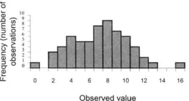
The most popular tool is the histogram. To begin with, assume that a discrete character is observed (to help in the presentation, it takes integer values , , , etc.). Let be the
Figure 1: Histogram, showing results of observations for a discrete variable
The outcome has been " " for element, while elements exhibit the value " ", and an average around " " can be guessed. Abnormal measurements may be discovered in this way
(here, perhaps " ", but the sample size is far too small for such a firm statement).
The case of continuous variables calls for a more careful analysis. The previous approach is no longer valid, as the outcomes are real numbers, scattered throughout the axis, with no two
identical values. The method is to group the observations in classes and to draw cumulated frequencies. intervals are defined: , . They are usually referred to as bins. Class bin gathers all observations within interval , and contains observations: ??? ( , such
that ). With for the size of the whole population, the relative frequency for class
is the ratio . The curve of cumulated frequencies displays the whole set of measurements:
, for , .
The curve is made up of a series of horizontal segments (Figure 2).
The histogram is another representation, just as for discrete value observations, provided that the "area rule" is observed. For each interval , a rectangle is constructed with a base length
equal to its range and an area proportional to the number of observations within the
interval. This guarantees the validity of the interpretation given to the graph:
Class is represented on the histogram by a rectangle with area (instead of height) proportional to . For bins of equal width, the distinction makes no sense. In the general case, the rule is motivated by the following arguments:
1. It allows interpretation of the ordinate as an "empirical density".
2. It allows an unbiased comparison between frequencies of the different classes to be made.
3. It makes the histogram insensitive to class modifications (especially, the shape remains the same if several bins are grouped).
Other representations
Numerous other description tools have been imagined, the goal of which is to provide a synthetic, intuitive, access to the set of data. Various software packages make them easy to use.
2.1 Histogram
In statistics, a histogram is a graphical display of tabulated frequencies, shown as bars. It shows what proportion of cases fall into each of several categories: it is a form of data binning. The categories are usually specified as non-overlapping intervals of some variable. The categories (bars) must be adjacent. The intervals (or bands, or bins) are generally of the same size.
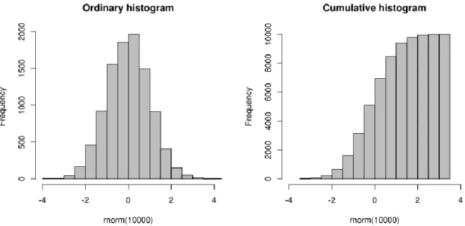
Histograms are used to plot density of data, and often for density estimation: estimating the probability density function of the underlying variable. The total area of a histogram used for probability density is always normalized to . If the length of the intervals on the -axis are all ,
Figure 3: An ordinary and a cumulative histogram of the same data. The data shown is a random
sample of points from a normal distribution with a mean of and a standard deviation of
.
Mathematical definition
In a more general mathematical sense, a histogram is a mapping that counts the number of observations that fall into various disjoint categories (known as bins), whereas the graph of a histogram is merely one way to represent a histogram. Thus, if we let be the total
number of observations and be the total number of bins, the histogram meets the following
conditions:
.
Cumulative histogram
A cumulative histogram is a mapping that counts the cumulative number of observations in all of the bins up to the specified bin. That is, the cumulative histogram of a histogram
is defined as:
.
Number of bins and width
methods generally make strong assumptions about the shape of the distribution. You should always experiment with bin widths before choosing one (or more) that illustrate the salient features in your data.
The number of bins can be calculated directly, or from a suggested bin width :
.
The braces indicate the ceiling function.
3 Statistical parameters
The direct visualization of the data is a first and important step. At that point, the need arises for a quantitative characterization for the parameter of interest. Here again, the assumption is that statistical laws, often difficult to identify, govern the phenomena under study. To begin with, one makes use of global parameters that introduce no specific assumption about the underlying probabilistic models.
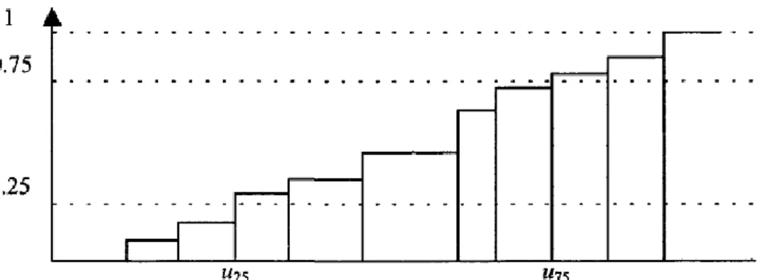
3.1 Fractiles
Fractiles are read directly on the cumulated frequency curve. Let be the cumulated frequency of variable : is the ratio of measured values equal to or less than . The
-fractile (also referred to as quantile or percentile) is the number such that , .
This notion may help eliminate extreme values, most often abnormal. In the common situation where the measured character has no upper bound, the range of interest can be chosen as the interval between the -fractile and -fractile. In economics use is made of
quartiles (values for , or ). The -fractile is called median. It divides the whole
Figure 4: Fractiles of a distribution function
3.2 The sample mean
Among the global numeric indicators that are derived from the raw data, the mean value (or average) is certainly the most popular. The term empirical mean is sometimes used to emphasize the fact that this quantity is estimated, as opposed to the theoretical mean value of a probabilistic distribution. It is most commonly denoted as :
,
being the sample size.
3.3 The sample variance
In order to represent the dispersion (intuitively the distance from the average behaviour given by the sample mean), the sample variance is introduced:
.
The standard deviation is the square root of the variance.
3.4 The moments
The -moment of the distribution (moment of order ) is usually denoted as . Most
.
(the first moment is ).
3.5 The mode
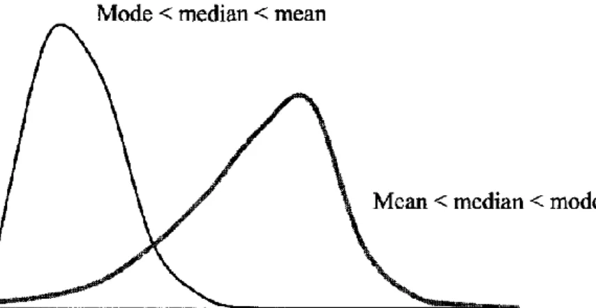
The mode is the most frequently observed value. It is given by the maximum of the histogram. Distributions with a single mode are referred to as being unimodal.
Mode, median and mean values must be carefully distinguished. The mode is visible on the histogram; the median separates the population in two subsets of equal size, and the mean in two subsets of equal "weight". Unimodal distributions fit in one of the two categories:
mode < median < mean (the distribution is spread to the right);
mean < median < mode (the distribution is spread to the left).
Figure 5: Mean, mode, median of a density function
3.6 Other characterisations
The mean and variance do not capture all features of the distribution. Other indicators have been proposed, which take account of certain classes of shapes of the distribution functions. These indicators are derived from the moments. Here too these indicators are to be seen as "empirical" (i.e. defined from the sample). In order to simplify the notations, the "–" are omitted in what follows.
These coefficients (respectively, Fisher and Pearson coefficient) reflect the skewness of the distribution. They take account of the symmetry the function may exhibit; they vanish when the curve is symmetric.
, .
These coefficients allow comparison of the peakedness of the distribution (the "kurtosis") with the normal distribution, which is such that , , and so