Thesis

Congestion Avoidance on Road Networks through Adaptive Routing on Contracted Graphs

by

Bradley H. Davis

A Senior Honors Thesis submitted in partial satisfaction of the

requirements for the degree of

Bachelor of Science in Computer Science

from the

Department of Computer Science

at

1

Abstract

i

This body of work is dedicated to

The James M. Johnston Trust for Charitable and Educational Purposes &

Mr. and Mrs. R. T. Davis of Greensboro, North Carolina

ii

Contents

Contents ii

List of Figures iii

List of Tables iv

1 Problem Origins 1

1.1 Modern Mapping Services . . . 1

1.2 The Secondary Congestion Problem . . . 3

1.3 A Driverless Future . . . 4

2 Finding the Shortest Path Quickly 6 2.1 Dijkstra’s Algorithm . . . 6

2.2 Decision Graphs . . . 8

2.3 Shortcuts . . . 8

2.4 Advanced Algorithms and Techniques . . . 10

3 Accelerating Graph Processing 12 3.1 Contraction Hierarchies . . . 12

3.2 Heuristics for Node Ordering . . . 14

3.3 Effects of Node Ordering . . . 16

4 Routing with Dynamic Edge Weights 19 4.1 Weight Function . . . 19

4.2 Simulation Environment . . . 20

5 Findings 23 5.1 Experiments . . . 23

5.2 Results . . . 24

5.3 Concluding Remarks . . . 27

5.4 Future Work . . . 27

iii

List of Figures

2.1.1 Search Space of Dijkstra’s Algorithm . . . 7

2.1.2 Search Space of Bidirectional Dijkstra’s Algorithm . . . 7

2.2.2 A Decision Graph . . . 9

2.3.2 A Graph with Shortcuts . . . 9

3.1.4 A Node Order . . . 14

3.1.5 A Contraction Hierarchy . . . 15

3.3.2 Effects of Node Ordering on Contraction Time . . . 17

3.3.4 Effects of Node Ordering on Routing Speed . . . 18

4.2.1 Traffic Flow Model . . . 22

5.1.1 Simulation Visualization . . . 24

5.2.2 Adaptive Routing with 1,000 Single-Origin Single-Destination Routes . . . 25

5.2.3 Adaptive Routing with 10,000 Random-Origin Random-Destination Routes . . . 26

iv

List of Tables

3.3.1 Effects of Node Ordering on Contraction Time . . . 16

3.3.3 Effects of Node Ordering on Routing Speed . . . 17

4.2.2 List of Universal Simulation Parameters . . . 22

v

Acknowledgments

1

Chapter 1

Problem Origins

It is vitally important to provide some context in which this body of research was inspired and conducted. As early as 1996, companies such as MapQuest had begun to harness the nascent Internet to deliver online maps and driving directions [17]. In 2005, Google launched its own web mapping service for desktop computers and mobile phones; by 2009, it made turn-by-turn directions available on select smartphones [25]. Since then, a number of competing services have emerged. Feature sets have expanded to include arial photography, street-level photography, business directories, multimodal trip planning, and live traffic information. The overwhelming importance of these mapping services is becoming indisputable as popular services experience upwards of five billion requests per week [22].

In this chapter, we discuss the state of present-day mapping services and outline our idea that routing a large fleet of vehicles via shortest paths on static graphs produces unnecessary secondary congestion.

1.1

Modern Mapping Services

Quantitative Bases

Current mapping services work with a somewhat limited number of data sources collected directly or provided by third party providers. The following is a non-exhaustive list of information available to most services:

• length of road segments

• road classifications and free-flow speed estimates

• posted speed limits [16]

• scheduled road maintenance events

CHAPTER 1. PROBLEM ORIGINS 2

• crowdsourced reports of incidents

• historical information and predictions derived from the items above

It is unclear to what extent popular services utilize these sources of information. Presum-ably, a minimal basis for producing shortest-travel-time directions uses the product of road segment lengths and speed estimates to estimate trip durations.

Live Traffic Information

The way in which a mapping service makes use of traffic information can greatly improve the accuracy of routes produced. Publishing road conditions in the form of a color-coded map overlay can aid drivers in making decisions; deriving historical traffic trends is similarly helpful. Ideally, historical data could be used to predict traffic conditions although such predictions are limited by the frequency and reliability of measurements [2].

How a service acts on live information is also vital to producing better directions. If a service only calculates a route once at the inception of a trip, it risks making vehicles avoid impediments that may not exist by the time the vehicle reaches them. If routes are re-evaluated whenever congestion is encountered, there may be no viable alternatives or only globally suboptimal ones. Google in particular has recognized the plight of these approaches and since early 2014 has offered automatic rerouting [24].

Speed & Scope

One of the defining features of modern web mapping services is unparalleled performance at scale. Like many other types of web applications, these services consistently have to handle a large volume of queries quickly. Doing so is not only convenient for users waiting on the results, but important for making time-sensitive decisions like whether to reroute a moving vehicle. Although precise statistics about proprietary services are not easy to obtain, it is generally true that trans-American routes can be computed in less than a couple of seconds and shorter routes in a number of milliseconds.

CHAPTER 1. PROBLEM ORIGINS 3

1.2

The Secondary Congestion Problem

Definition

The root of our research activities lies in an experience that we believe to be fairly common when driving in the United States. This particular situation, which we call the Secondary Congestion Problem, illustrates some ways in which navigational decisions could be im-proved. It is described as follows:

Suppose you are traveling back from a weekend excursion in a foreign place and need to use your phone’s Internet-enabled mapping application to get directions home. Your phone provides turn-by-turn directions; you obey them strictly. At some point in your trip you find yourself traveling along an interstate highway at free-flow speed. Much to your chagrin, you suddenly come upon a congested section of road that is nearly at a standstill. After slowly rolling along for some time, you request an alternate route on your phone. The alternate route takes you off the interstate at the next exit and onto a two-lane road with a much lower speed limit. Five minutes into your detour, you have yet to reach free-flow speed as this road is also completely saturated with traffic. You wonder if this alternative route was really worth pursuing after all.

Proposed Solution

We have experienced the Secondary Congestion Problem more than once in real life. The recurrence of such an unpleasant experience drove us to ask the question "Why not provide vehicles with continuously updated routes to their destination that make good use of the wealth of information reported by other vehicles?" To this end, we envision a new web mapping service where:

• a vehicle receives route assignments from a central authority

• a vehicle records the time it takes to drive along each predefined segment of the road, and reports these durations to the central authority using an Internet connection

• the central authority uses the reports to quickly update its model used for giving directions

• at critically frequent times, vehicles ask the authority for an updated route assignment

CHAPTER 1. PROBLEM ORIGINS 4

Luckily, the technology required is already available and widely adopted: cloud comput-ing makes centralized routcomput-ing authorities more possible than ever and new cars are often equipped with cellular radios for Internet connectivity. Costs would be low as well; no phys-ical traffic sensors would have to be deployed. We find this idea quite promising and hope that designing and modeling a realistic system with these goals in mind will yield an overall improvement in commute times.

Other Solutions

Aside from any of the aforementioned mapping services, there is at least one other existing service that shares a similar vein of thinking. Nunav, formerly Greenway, is a navigation application that re-evaluates routes every thirty seconds. Nunav estimates road capacities based on classification and actively balances its users so that no road becomes oversatu-rated [18]. Such an avant-garde approach is refreshing but has a seemingly critical flaw: it works best when Nunav controls all or nearly all traffic within a network.

Our concept does not attempt to calculate the capacity of a particular road. Instead, it solely uses changes in the duration of traversal. This means that if a lane is suddenly blocked, we will not overestimate the capacity of the road at that time. Further, the ability to make decisions based on a small sample of vehicles means that our approach would be suitable for the period of time between present day and a time at which nearly all vehicles are using our mapping service.

1.3

A Driverless Future

Autonomous Vehicles

Vehicles that can operate without human intervention or presence were once a figment of fan-ciful thinking. Today, autonomous vehicles are an imminent disruption in the way we travel — one that is simultaneously miraculous and frightening. Most major automobile manufac-turers are already working on semi or fully autonomous cars that utilize some combination of laser, radar, and optical cameras [11]. In fact, some of these vehicles are already legal and currently deployed on roads throughout the United States [7]. By 2022, basic automated systems such as automatic braking will be standard feature on almost every vehicle [21].

CHAPTER 1. PROBLEM ORIGINS 5

• offline map data quickly becomes outdated and is difficult to update without use of the Internet

• on-board route computations are performance-bound by installed hardware and such hardware is difficult to upgrade

• integrating live traffic information into an offline routing system would likely require peer-to-peer vehicle communication, which is inherently complex and suffers from lo-cality problems

Effects on Our Research

6

Chapter 2

Finding the Shortest Path Quickly

Finding the shortest path in a large graph is not an easy task — a graph of roads in the continental United States has 24 million nodes and 29.1 million edges [1]. In this chapter we examine existing various techniques that prune search space, reduce graph size, and employ heuristics to speed up queries.

2.1

Dijkstra’s Algorithm

An exceptionally straightforward approach to finding the shortest path in a graph with positive edge weights was described by Edsger W. Dijkstra in 1956 [9]. Dijkstra’s algorithm, as it is called, starts at the origin node s of a query and adds all neighboring nodes ns to a

queue sorted by distance from s to ns. While the queue has elements and the destination

nodethas not yet been encountered, a node is popped from the queue and all of its neighbors are enqueued with their shortest distances from s to that node.

In the original implementation, Dijkstra’s algorithm for a graph G = (V, E) runs in quadraticO(|E|2_{). This is highly problematic at scale; if each step completed in 1 picosecond,}

a worst-case search on the United States road network would take roughly 15 minutes to complete.

Bidirectional Dijkstra’s Algorithm

CHAPTER 2. FINDING THE SHORTEST PATH QUICKLY 7

Figure 2.1.1: The search space required by Dijkstra’s algorithm to find the red path is shown in blue.

CHAPTER 2. FINDING THE SHORTEST PATH QUICKLY 8

2.2

Decision Graphs

Since most pathfinding algorithms’ performance is bounded in some way by |V| or|E|, it is always in our best interest to reduce the size of the graph. Graphs of road networks often contain excess vertices and edges that represent physical geometry which are not useful for producing a set of driving directions. In our case, we can reduce a graph to only the set of nodes and edges that correspond to ‘decisions’ a driver could make: making a turn, taking an exit ramp, etcetera. We refer to such a graph as a decision graph, which is a concept frequently employed to distill complex decision trees [20].

Algorithm 2.2.1 Reducing a full-sized graph into a decision graph

1: function decision_graph(G) 2: for all v ∈VG do

3: P ← {u∈VG | hu, vi ∈EG}

4: S← {w∈VG | hv, wi ∈EG}

5: if (|P|= 2∧ |S|= 2)∨(|P|= 1∧ |S|= 1) then

6: for all (hu, vi,hv, wi)∈P ×S do

7: EG ←EG− {hu, vi,hv, wi}+{hu, wi}

8: end for

9: VG ←VG− {v}

10: end if

11: end for

12: end function

2.3

Shortcuts

Shortcuts are introduced edges that act as summaries of paths in G [5]. Adding shortcuts to a graph may significantly increase |E|, but can also greatly reduce the number of nodes settled during a Dijkstra search.

Definition 2.3.1 (Shortcut). A shortcut hx, yi ∈ E is an edge such that for some path

P ⊂E from x to y, |hx, yi|=P

CHAPTER 2. FINDING THE SHORTEST PATH QUICKLY 9

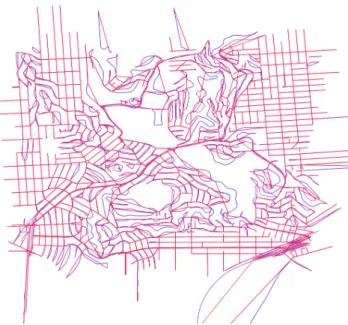
Figure 2.2.2: A full-sized graph in blue overlaid with its corresponding decision graph overlaid in red.

CHAPTER 2. FINDING THE SHORTEST PATH QUICKLY 10

2.4

Advanced Algorithms and Techniques

There are two additional ways to improve the performance of Dijkstra’s algorithm: discarding nodes that are not helpful in a given search and prioritizing ones that are more likely to be helpful. Dijkstra-based search algorithms prioritize nodes closest to the current node, but often better results are possible by directing the search towards a goal. The next two techniques employ an admissible potential function to improve search efficiency.

Definition 2.4.1 (Potential Function). A potential function π(v, t) is a function estimates that the cost of traveling from vertex v ∈V to terminal vertex t∈V on a given graph G. Definition 2.4.2(Admissibility). A potential functionπ is admissible if and only if it never overestimates the cost of traveling from vertex v ∈ V to terminal vertex t ∈ V on a given graph G.

A*

A* search is a simple extension of Dijkstra’s algorithm that adds the result of a potential functionπ(v, t) to the sort order, whereπ(v, t) is an estimate of the distance fromv to query destination t. This allows nodes that make large advances toward the destination to be prioritized over nodes that are nearby but stray away from the ultimate goal. However, a great deal of care has to be taken to maintain optimality; only admissible heuristics return optimal routes.

Some specific problems include pertinent information that is useful for constructing a good potential function. For example, the physical distance between nodes in a road network graph can be used to as a heuristic for shortest-distance queries [27] This is more generally known as Euclidean-based A*.

ALT

A*, Landmark, and Triangle Inequality (ALT) are a class of algorithms that combine A* search with the principles of a bidirectional Dijkstra’s algorithm. ALT selects a set of land-marks and computes the shortest path from each vertex to and from the landmark. Using the triangle inequality, it then ensures that any value returned by the potential function is an underestimate of the distance remaining to a goal node [13]. Thus the potential function is an admissible heuristic for A*.

A*-based approaches are effective at prioritizing important nodes but there is still the potential to further improve queries by pruning less promising paths.

Reach

CHAPTER 2. FINDING THE SHORTEST PATH QUICKLY 11

Intuitively, the reach of a vertex encodes the lengths of shortest paths on which it lies. To have a high value of reach, a vertex must lie on a shortest path that extends a long distance in both directions from the vertex. [15]

Reach can be combined with ALT and shortcuts to produce REAL, which further improves query times [14].

Arc Flags

A graphGcan be divided intok partitions{P0, ...Pk}that are roughly uniform in size. Each

edge hu, vi has a flag for each of the partitions, indicating whether the edge is useful for reaching a destination in that partition [6]. Furthermore, arc flags can be combined with shortcuts to yield SHARC, which can be useful for unidirectional searches in graphs that are time-dependent [4].

Hierarchies

An elegant algorithm for finding shortest paths was published by Robert Geisberger in 2008 at the Institut für Theoretische Informatik Universität Karlsruhe [12]. His work builds upon Dominik Schultes’ dissertation on Highway Hierarchies [23]. Highway Hierarchies combine shortcuts and pruning to create a hierarchy of overlay graphs based on assigned importance. This works nicely with categorical data such as map data since roads are often classified into a handful of categories such as motorway, primary, secondary, and residential.

Geisberger’s generalization assigns each vertex in a graph to its own level in the overlay hierarchy. Contraction Hierarchies (CH) use bidirectional Dijkstra’s algorithm and shortcuts, but can also incorporate other techniques including, but not limited to, arc flags (CHASE). After considering all of the above, we chose to apply this approach to our research for a few important reasons:

• recency of the concept

• query performance

• elegance and relative simplicity

12

Chapter 3

Accelerating Graph Processing

Graph processing techniques that take minutes or hours on large graphs are inherently unsuitable for graphs with dynamic weights. In this chapter we describe our contribution to refining one of these techniques and subsequently its effects on query speeds.

3.1

Contraction Hierarchies

Definition

Definition 3.1.1 (Contraction Hierarchy). C(G) = (H, <) is a contraction hierarchy of an input graph G= (V, EG), where <is a total order on V, H = (V, EH), (EH ⊇EG), and

(∀hu, wi ∈(EH −EG)∃v ∈V | hu, vi ∈EH ∧ hv, wi ∈EH ∧ |hu, vi|+|hv, wi|=|hu, wi|)

Definition 3.1.2 (Remaining Graph). G↑v is the remaining graph of a node v.

G↑v = (VG↑v, EG↑v) = ({u∈VG |u > v},{hu, wi ∈EG |u > v∧w > v})

Contracting a graph G involves ordering all nodes v ∈ V and constructing a graph H

which shares the same set of nodes and a superset of edges. Any edgeeH added toH during

the process, called a shortcut, has a length equal to the sum of the lengths of two other adjacent edges: one that shares an initial point with eH and one that shares a terminal

point. The algorithm used to query H is a bidirectional variant of Dijkstra’s algorithm with a constraint that only nodes in the remaining graph can be relaxed. This prunes a large portion of the search space and is the heart of what contraction hierarchies have to offer.

Procedure

The general procedure for producing a contraction hierarchy is simple and yet computation-ally complex. First, all nodes must be ordered according to a heuristic. Then, each node v

CHAPTER 3. ACCELERATING GRAPH PROCESSING 13

path from u to w for each pair of neighbor nodes hu, vi hv, wi in G↑v. If no shortest path is found, or the shortest path is hu, vi+hv, wi, then a shortcut edge hu, wi must be added. Before the next node is contracted, all un-contracted nodes must be reordered.

Algorithm 3.1.3 Simple approach to contracting a graph

1: function _order(Q)

2: for all (k, v)∈Qdo

3: k← _heuristic(v)

4: end for

5: _heapify(Q)

6: end function

7: function _contract(G)

8: EH ←EG

9: i←0

10: Q← {(∞, v)|v ∈V}

11: _order(Q)

12: while Q do

13: k, v←Q.pop()

14: for all u∈VG↑n do

15: for all w∈VG↑n |u6=w do

16: path ←_{local_search}(u,v,w)

17: if |path| ≥ |hu, vi|+|hv, wi|then

18: EH ←EH ∪ hu, wi

19: end if

20: end for

21: end for

22: _order(Q)

23: end while

24: return H = (V, EH)

25: end function

Basic Optimizations

In the contraction algorithm above, _{local_search} is the aforementioned Dijkstra search and_heapifyis a function to sort a set of tuples (k, v) by k. Since_{local_search} is buried inside nested inside aO(|VG↑n|2) operation, it clearly has a strong effect on contraction speed.

There are many optimizations that we could apply to the local Dijkstra search:

• limit the number of settled nodes [12]

CHAPTER 3. ACCELERATING GRAPH PROCESSING 14

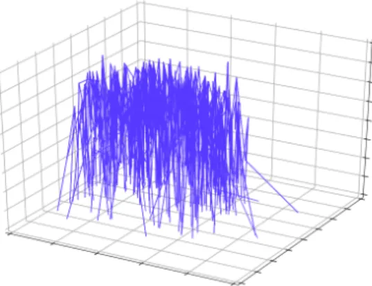
Figure 3.1.4: A visualization of a graph after its nodes have been ordered. The z-axis corresponds to node order.

• forgoing Dijkstra’s algorithm in favor of a simple scanning search whenever a small hop limit is imposed [12]

• reducing the number of edges by removing original edges hu, wi if |hu, wi|>|hu, vi|+

|hv, wi| when v is being contracted [12]

• implementing Dijkstra’s algorithm with a Fibonacci heap, which provides O(|E|+

|V|log|V|) performance [10]

• ensuring edge weights are positive integers and multiplying in linear time, which pro-videsO(|E|) performance [26]

Each of these optimizations would likely improve the overall speed of contraction. However, dynamic analysis indicates that the runtime of _contract is in fact dominated by _order. One improvement that can reduce the effect of calls to _order is choosing to only run

heuristicon neighbors of the most recently contracted node. This has little impact on the

quality of the contraction and a large impact on contraction speed [12].

3.2

Heuristics for Node Ordering

EDS5

Definition 3.2.1 (Edge Difference). The edge difference of a noden is the number of short-cuts that must be added to contract n, less the number of edges that will be removed from the remaining graph.

CHAPTER 3. ACCELERATING GRAPH PROCESSING 15

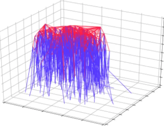
Figure 3.1.5: A visualization of a contraction hierarchy where shortcut edges are shown in red and the z-axis corresponds to node order.

simple; the fewer shortcuts that must be added and the greater the number of edges removed, the sooner a node should be contracted. Many heuristics containing the edge difference term were profiled and among the best was a heuristic referred to as EDS5.

Definition 3.2.2 (EDS5). The priority of a node n is given by

heuristic(n) =E+D+S

where E is the edge difference obtained by simulating a contraction of n, D is the number of nodes adjacent to n that have been contracted, S is the size of the search space required to determine the edge difference, and _{local_search} was performed with a 5-hop limit.

N5

Definition 3.2.3 (N). NG↑v is the set of neighbors in the remaining graph.

NG↑v ={u∈G↑v |(hu, vi ∈EG)∨(hv, ui ∈EG)}

The goal of previously defined node ordering heuristics is to minimize query times while providing reasonable contraction times. Our goal, however, is to minimize contraction times while providing reasonable query times. If we are to integrate new traffic information as quickly as possible, and thus calculate new edge weights often, this optimization is abso-lutely essential. Contracting a node with a heuristic such as EDS5 is a O(|NG↑v|2|EG↑v|2)

operation, since for every pair of neighbors in the remaining graph NG↑v, we must do a

Di-jkstra search of as many as |EG↑v|edges. Any improvements made to order would greatly

reduce contraction time, since it is called many times per node.

CHAPTER 3. ACCELERATING GRAPH PROCESSING 16

define our heuristic, we took this idea to its logical extreme and attempted to reduce node priority calculation to a linear time operation.

Definition 3.2.4 (N5). The priority of a node n is given by

heuristic(n) = |NG↑n|

N5 prioritizes nodes that have the fewest remaining neighbors so that nodes which require many runs of _{local_search} are contracted last. Contracting nodes with a high degree often leads to the creation of many shortcuts since road networks can be sparse or have significantly varying weights (due to differing road classifications). Delaying the addition of as many shortcuts as possible reduces the chance that one of those shortcuts will become a neighbor for a later node that must be evaluated during contraction. The biggest advantage of N5, however, is that evaluating |NG↑n| is an O(|EG↑n|) operation. This is a significant

improvement since N5 entirely forgoes using a Dijkstra search within _heuristic.

3.3

Effects of Node Ordering

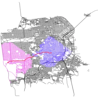
We studied the effects of our heuristic on both full-sized graphs and their equivalent decision graphs of successively larger maps centered about the SOMA district of San Francisco, California. Map sizes ranged from a few blocks to the entirety of the San Francisco Bay Area. By timing the contraction process and the mean routing speed of 5,000 random route queries, we highlight the trade-offs of using N5 as a node ordering heuristic.

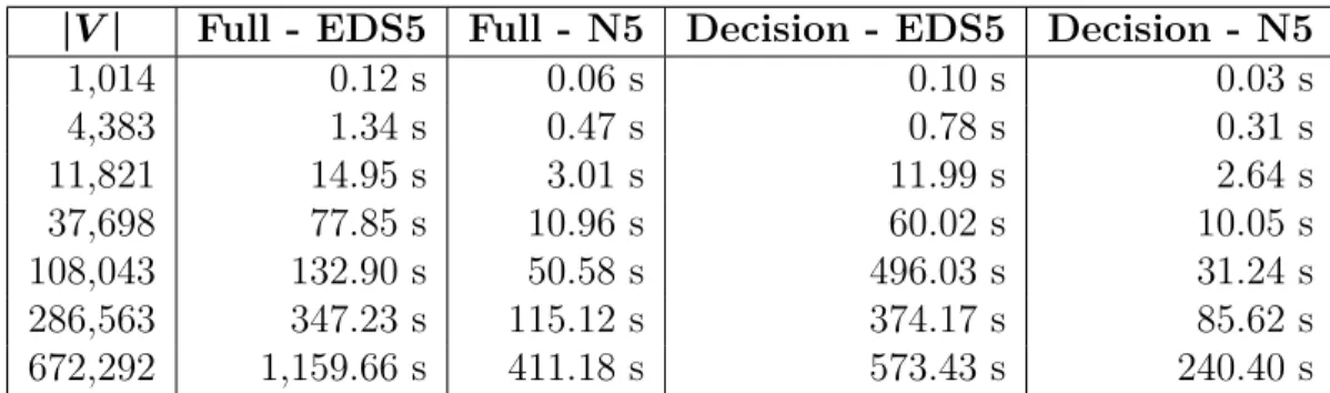
On Contraction Time

It is apparent in the figure below that using our novel N5 heuristic allows graphs to be contracted more quickly than when using EDS5. Furthermore, the results confirm that reducing the size of the input graph yields a predictable savings in contraction time over usage of a full-sized graph.

|V| Full - EDS5 Full - N5 Decision - EDS5 Decision - N5

1,014 0.12 s 0.06 s 0.10 s 0.03 s

4,383 1.34 s 0.47 s 0.78 s 0.31 s

11,821 14.95 s 3.01 s 11.99 s 2.64 s

37,698 77.85 s 10.96 s 60.02 s 10.05 s

108,043 132.90 s 50.58 s 496.03 s 31.24 s

286,563 347.23 s 115.12 s 374.17 s 85.62 s

672,292 1,159.66 s 411.18 s 573.43 s 240.40 s

CHAPTER 3. ACCELERATING GRAPH PROCESSING 17

Figure 3.3.2: A chart of the relative preprocessing performance of N5.

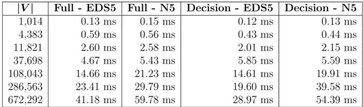
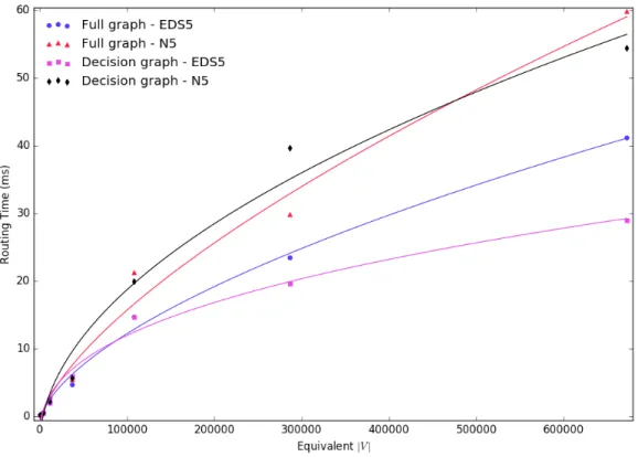
On Routing Speed

These results confirm the intuition that N5 would harm query speed. Given the context of our research, these slower speeds are still quite suitable for city or intrastate routing. The reduction in graph size afforded by the decision graph does not appear to affect N5 performance, but makes EDS5-based routing even faster.

|V| Full - EDS5 Full - N5 Decision - EDS5 Decision - N5

1,014 0.13 ms 0.15 ms 0.12 ms 0.13 ms

4,383 0.59 ms 0.56 ms 0.43 ms 0.44 ms

11,821 2.60 ms 2.58 ms 2.01 ms 2.15 ms

37,698 4.67 ms 5.43 ms 5.85 ms 5.59 ms

108,043 14.66 ms 21.23 ms 14.61 ms 19.91 ms

286,563 23.41 ms 29.79 ms 19.60 ms 39.58 ms

672,292 41.18 ms 59.78 ms 28.97 ms 54.39 ms

CHAPTER 3. ACCELERATING GRAPH PROCESSING 18

Figure 3.3.4: A chart of the relative routing performance of N5.

On Number of Edges

19

Chapter 4

Routing with Dynamic Edge Weights

In order to use our modified routing algorithm in conjunction with live traffic information reported by autonomous vehicles, we must find a way to reduce some set of travel times into a single value that can act as an edge weight. In this chapter, we define our function for computing edge weights and describe our experimental setup.

4.1

Weight Function

An edge weight should ideally always represent travel times at the exact moment of the route query. This is wholly infeasible in practice because:

• there no guarantee of when or how many reports will be received

• reports will naturally conflict due to different speeds, driving styles, road conditions, etc.

• any given report could be erroneous

Using a moving average for compiling conflicting reports would be straightforward. Un-fortunately, a moving average requires a window over which reports are averaged. This is problematic; as we lengthen the window to reach an accurate average, we dampen the effect of recent reports. If the window were one hour, for example, then a single report detailing a sudden slowdown on a road is unlikely to raise the moving average quickly enough to warn other vehicles.

Definition 4.1.1 (Updating Graph Weights). Let wt =|hu, vi| of an edge hu, vi at time t.

When the graph is updated at time t+ 1:

wt+1 =

  

λRt+ (1−λ)wt if |R|>0

max(λδwt+ (1−λ)wt, w0) otherwise

where λ∈[0,1] is the smoothing factor, δ∈ [0,1] is the decay factor, and Rt⊂R is the set

CHAPTER 4. ROUTING WITH DYNAMIC EDGE WEIGHTS 20

Exponential Smoothing

Instead of a moving average, we chose to average the reports within an update period and use exponential smoothing to aggregate traffic reports across update periods. Exponential smoothing is simple in principle and efficient in practice. First, we choose a value for the smoothing factor λ ∈ [0,1]. On each graph update, the new weight for an edge is λ parts the mean of the reports for that edge received since the last update and 1 −λ parts the previous edge weight. This strategy means that we can control how much of an impact a recent change in travel times has on our route calculations.

Exponential Decay

If vehicles report a spike in travel times indicative of a near-standstill, our system should start rerouting all approaching vehicles. This is desired behavior. Yet if no approaching vehicles to take the blocked path, our system thus far will fail when the congestion clears. No reports of improved travel times means that vehicles will be permanently rerouted around a temporary obstacle.

To account for this scenario we introduce a decay parameter δ ∈ [0,1] that linearly reduces the weight of an edge each update period that no reports are received for that edge. If the weight of such an edge reaches its original value from when the graph was initialized, we cease the decay process. Recall that calculated edge weights are exponentially smoothed, so linear decreases smoothed over successive update periods are also exponential.

Graph Updates

Contraction Hierarchies are intended to be a preprocessing technique. With our adaptations in place, we repeatedly run the preprocessing step — we will hereafter refer to it as simply ‘processing’. Processing a graph consists of removing all shortcuts, calculating a new weight for all original edges using newly received reports, and then running _contract.

There are many potential optimizations that can be made to this process, including keeping shortcuts whose constituent edges are unaffected by an update and reusing the node order from previous contractions. We elected not to implement these for simplicity’s sake.

4.2

Simulation Environment

CHAPTER 4. ROUTING WITH DYNAMIC EDGE WEIGHTS 21

Map Data

Map data was obtained from OpenStreetMapR _{in XML format and parsed in the following} way:

• road segments were presumed to be bidirectional unless explicitly marked as a one-way street

• all road segments were treated as comprising of a single lane in each direction

• latitude and longitude coordinates were used to calculate segment lengths

• road classifications were used to estimate free-flow speed

• segment lengths and free-flow speed were used to estimate the expected time to traverse a road segment; this value was used as a default edge weight

• segments were divided into car-length cells for simulation purposes

• signalized intersections were created only where explicitly marked

Signalized Intersections

OpenStreetMapR _{data on signal placement is not standardized: sometimes a single node is} marked as having a signal and other times each terminal node within a region are considered signals. Therefore, signals within one graph hop of another signal were considered to be part of an intersection and governed by a single instance of a control algorithm. Any inbound edges with matching street names were grouped together and added to a green light rotation. The control algorithm looped through each set of edges in the rotation for a fixed amount of time unless oncoming traffic was detected, in which case the time was extended until either the oncoming traffic ceased or a maximum timeout was reached.

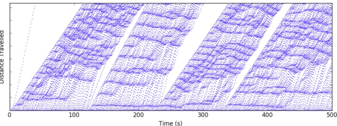
Vehicular Behavior

Each directed road segment was treated as a cellular automaton where only a single vehicle could occupy a given cell at any given time. Vehicle behavior along this one-dimensional automaton was modeled using a derivative of the Nagel-Schreckenberg model [19] in which vehicles attempted to maintain a particular amount of headway based on their current speed. Each vehicle was assigned a normally distributed speed adjustment factor to represent vari-ations in intended speed (e.g. drivers who wish to speed). A vehicle’s maximum acceleration was adjusted by a normally distributed factor to produce variations from different types of vehicles. Drivers were given a reaction time such that if a stopped car became able to move, its driver would notice within the reaction time period.

CHAPTER 4. ROUTING WITH DYNAMIC EDGE WEIGHTS 22

Figure 4.2.1: A distance-time plot of 1,000 simulated vehicles along a single path.

Parameter Values

We made a best-effort attempt at selecting reasonable values for our simulation parameters. Below is the set of parameters common to all of our experiments.

Name Value

green light duration 30 s

maximum extended green light duration 40 s

speed adjustment factor N(free-flow speed,5 m/s)

maximum acceleration 2.8 m/s2

acceleration adjustment factor N(0,0.5 m/s2)

driver reaction time 200 ms

graph update frequency 15 s

exponential smoothing factor (λ) 0.5

linear decay factor (δ) 0.9

23

Chapter 5

Findings

In this chapter, we describe the experiments we conducted, remark on their outcomes, and discuss future work.

5.1

Experiments

For each of the following experiments, two simulations were run. The simulations were nearly identical; the same cars with the same varied parameters were spawned in the environment in the same order. The initial contracted graphs were identical and signals were started in a universal state. Vehicles reported the simulated duration of traveling along a road segment at the end of each edge. Vehicles also re-requested routes to their destination at every decision node, but one simulation did not update its graph and the other used the traffic reports to return adaptive routes. All simulations were run for a simulated half-hour. Our ultimate goal was to elucidate any statistical differences in commute time.

Single-Origin Single-Destination (SOSD)

The first experiment conducted was a fleet of 1,000 cars originating at a single node at a rate of 100 cars per minute and headed for a common destination. The graph was a section of Greensboro, North Carolina centered around the intersection of Pisgah Church Road and Battleground Avenue. This single-origin single-destination experiment was designed to force highway saturation and expose the resulting routing behavior at a microscopic level.

Random-Origin Random-Destination (RORD)

CHAPTER 5. FINDINGS 24

metropolitan simulation. An additional experiment was run this this environment with 100,000 cars spawning at 10,000 cars per minute.

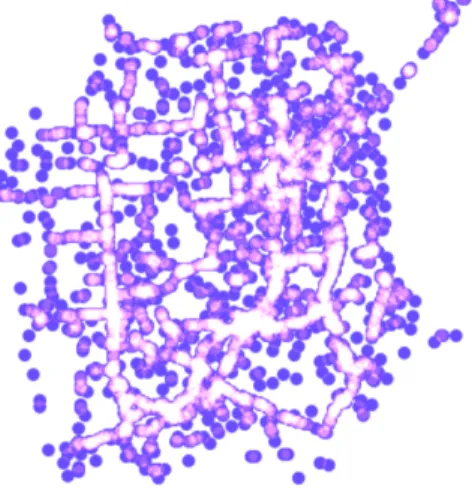
Figure 5.1.1: A visualization of one of the simulations run on the roads of San Francisco.

5.2

Results

At the end of each experiment, we collected the total driving time of every vehicle and discarded values from any vehicle that did not complete its intended journey in both the non-adaptive and adaptive simulations. Upon constructing histograms of travel times, we observed that the data was roughly normally distributed.

Simulation Cars Non-adaptive N(µ, σ) Adaptive N(µ, σ) Mean Speedup SOSD 1,000 N(1128.47,107663.16) N(1062.20,75063.76) 66.26 s RORD 10,000 N(637.37,124367.41) N(585.51,97453.41) 51.87 s RORD 100,000 N(232.74,42441.12) N(220.17,30939.65) 12.57 s

CHAPTER 5. FINDINGS 25

Figure 5.2.2: A normal probability density function showing the mean trip duration speedup for 1,000 cars traveling from a single origin to a single destination.

Our primary observation is that in all three experiments, enabling adaptive routing re-sulted in a reduction in mean trip duration of up to one minute. This is significant because it means that our simplistic method for computing edge weights combined with frequent route recomputation led to a higher likelihood of a faster trip for all vehicles. While one minute may seem insignificant, it is important to note that there is an upper bound on how much a commute can be sped up: theoretically determined by the straight-line distance and top speed, and realistically determined by available roads and traffic behaviors.

CHAPTER 5. FINDINGS 26

Figure 5.2.3: A normal probability density function showing the mean trip duration speedup for 10,000 cars traveling from a random origin to a random destination.

CHAPTER 5. FINDINGS 27

5.3

Concluding Remarks

We have presented a novel node ordering heuristic for a modern graph processing technique that allows for rapid edge weight mutations on graphs of metropolitan scale. Collecting a single metric from all vehicles within a road network in a manner that is feasible with today’s technology is sufficient for improving commute times using our elementary function for computing edge weights. Our mapping service design is appropriate for both immediate implementation with smartphones and future implementation with autonomous vehicles.

5.4

Future Work

Improving simulation quality is a high priority for any future work. Overtaking (passing) is a common phenomenon on roads with multiple lanes and is something that should undoubtedly be included in a traffic model. More realistic signal control algorithms are also important, especially in areas where signals are networked to provide coordinated state transitions. Additionally, varying vehicle length would be a welcome addition.

Our implementation of Contraction Hierarchies should also be improved. While Python was an appropriate choice for simulation, our implementation was not competitive with re-sults from the original paper on the topic. Using a lower-level language and focusing on implementing all previously defined optimizations may further reduce routing times. Ad-ditionally, combining N5 with arc flags for a CHASE routing variant might be a potential avenue for exploration.

28

Bibliography

[1] I. Abraham et al. A Hub-Based Labeling Algorithm for Shortest Paths on Road Net-works. Tech. rep. MSR-TR-2010-165. Microsoft Research Silicon Valley, 2010.

[2] K. Ashok. “Estimation and Prediction of Time-Dependent Origin-Destination Flows”. PhD thesis. Massachusetts Institute of Technology, Sept. 1996.

[3] D. Barth.The bright side of sitting in traffic: Crowdsourcing road congestion data. 2009.

url: https://googleblog.blogspot.com/2009/08/bright-side-of-sitting-in-traffic.html(visited on 04/10/2016).

[4] R. Bauer and D. Delling. “SHARC: Fast and robust unidirectional routing”. In:Journal of Experimental Algorithmics (JEA)14 (2009), p. 4.

[5] R. Bauer et al. “The Shortcut Problem–Complexity and Approximation”. In:SOFSEM 2009: Theory and Practice of Computer Science. Springer, 2009, pp. 105–116.

[6] M. Baum. “On Preprocessing the Arc-Flags Algorithm”. PhD thesis. Institute of The-oretical Computer Science Department of Informatics, 2011.

[7] R. Bradley. Tesla Autopilot. 2016. _url: https : / / www . technologyreview . com / s / 600772 / 10 - breakthrough - technologies - 2016 - tesla - autopilot/ (visited on 04/14/2016).

[8] J. Chang. Making the Shortest Path Even Quicker. 2009. _url: http : / / research . microsoft . com / en - us / news / features / shortestpath - 070709 . aspx (visited on 04/19/2016).

[9] E. W. Dijkstra. “A note on two problems in connexion with graphs”. In: Numerische Mathematik 1.1 (), pp. 269–271. _issn: 0945-3245. _doi: 10 . 1007 / BF01386390. _url: http://dx.doi.org/10.1007/BF01386390.

[10] M.L. Fredman and R.E. Tarjan. “Fibonacci Heaps And Their Uses In Improved Net-work Optimization Algorithms”. In: 2013 IEEE 54th Annual Symposium on Founda-tions of Computer Science(1984), pp. 338–346._doi:http://doi.ieeecomputersociety. org/10.1109/SFCS.1984.715934.

BIBLIOGRAPHY 29

[12] R. Geisberger. “Contraction Hierarchies: Faster and Simpler Hierarchical Routing in Road Networks”. PhD thesis. Institut fur Theoretische Informatik Universitat Karl-sruhe, July 2008.

[13] A. V. Goldberg and C. Harrelson. Computing the Shortest Path: A* Search Meets Graph Theory. Tech. rep. MSR-TR-2004-24. Vancouver, Canada: Microsoft Research, July 2004, p. 25. _url: http : / / research . microsoft . com / apps / pubs / default . aspx?id=64511.

[14] A.V. Goldberg, H. Kaplan, and R.F. Werneck. “Reach for A*: Efficient Point-to-Point Shortest Path Algorithms”. In: SIAM Workshop on Algorithms Engineering and Ex-perimentation (ALENEX 06). MSR-TR-2005-132. Miami, FL: Society for Industrial and Applied Mathematics, Jan. 2006, p. 41._url:http://research.microsoft.com/ apps/pubs/default.aspx?id=60764.

[15] R. J Gutman. “Reach-Based Routing: A New Approach to Shortest Path Algorithms Optimized for Road Networks.” In: ALENEX/ANALC 4 (2004), pp. 100–111.

[16] J. H. What speed does Google Maps use for drive time calculations. 2009._url: https: / / productforums . google . com / forum / # ! topic / maps / 3UhpvcDv24A (visited on 04/10/2016).

[17] AOL Inc. MapQuest Kicks Off Its 15th Year With Bright Future of New Products, a Hiring Push and Re-invigorated Consumer Experience. 2011._url:http://corp.aol. com/2011/04/25/mapquest-kicks-off-its-15th-year-with-bright-future-of-new-produ/ (visited on 04/10/2016).

[18] R. Metz.An App that Could Stop Traffic. 2012._url:https://www.technologyreview. com/s/428523/an-app-that-could-stop-traffic/(visited on 04/10/2016).

[19] K. Nagel and M. Schreckenberg. “A cellular automaton model for freeway traffic”. In: J. Phys. I France 2.12 (1992), pp. 2221–2229. _doi: 10.1051/jp1:1992277. _url: http://dx.doi.org/10.1051/jp1:1992277.

[20] J. J. Oliver. Decision Graphs — An Extension of Decision Trees. Tech. rep. 92/173. Monash University Department of Computer Science, 1992.

[21] J. F. Peltz. Automakers agree to make automatic braking a standard feature by 2022. 2016. _url: http://www.latimes.com/business/autos/la- fi- hy- auto- safety-20160317-story.html (visited on 04/15/2016).

[22] Associated Press. Apple Maps, once a laughingstock, now dominates iPhones. 2015.

url: http : / / www . betaboston . com / news / 2015 / 12 / 07 / apple maps once a -laughingstock-now-dominates-iphones/ (visited on 04/10/2016).

[23] D. Schultes. “Route Planning in Road Networks”. PhD thesis. Fakultat fur Informatik der Universitat Fridericiana zu Karlsruhe, Feb. 2008.

BIBLIOGRAPHY 30

[25] The Google Maps Team. Today we turn 10! 2015. _url: https://maps.googleblog. com/2015/02/today-we-turn-10.html(visited on 04/10/2016).

[26] Mikkel Thorup. “Undirected Single-source Shortest Paths with Positive Integer Weights in Linear Time”. In: J. ACM 46.3 (May 1999), pp. 362–394. _issn: 0004-5411. _doi: 10.1145/316542.316548._url: http://doi.acm.org/10.1145/316542.316548.