Mining emerging massive scientific sequence data using block-wise decomposition methods

(1)

Mining Emerging Massive Scientiﬁc Sequence Data

using Block-wise Decomposition Methods

Qi Zhang

A dissertation submitted to the faculty of the University of North Carolina at Chapel Hill in partial fulﬁllment of the requirements for the degree of Doctor of Philosophy in the Department of Computer Science.

Chapel Hill 2009

Approved by:

Wei Wang, Advisor

Leonard McMillan, Co-principal Reader

Jan Prins, Co-principal Reader

Fernando Pardo Manuel de Villena, Reader

(2)

c 2009 Qi Zhang

(3)

Abstract

Qi Zhang: Mining Emerging Massive Scientiﬁc Sequence Data using Block-wise Decomposition Methods.

(Under the direction of Wei Wang.)

I present eﬃcient data mining algorithms for knowledge discovery on two types of emerging

large-scale sequence-based scientiﬁc datasets: 1) static sequence data generated from SNP

diversity arrays for genomic studies, and 2) dynamic sequence data collected in streaming and

sensor network systems for environmental studies. The massive, noisy nature of the SNP arrays

and the distributive, online nature of sensor network data pose challenging issues for knowledge

discovery such as scalability, robustness, and eﬃciency. Despite the diﬀerent characteristics of

the SNP arrays and streaming sensor data, when viewed as sequences of ordered observations,

both can be eﬃciently mined using algorithms based on block-wise decomposition methods.

I present models and mining algorithms for inferring the genetic variation structure in

genome-wide Single-Nucleotide Polymorphism (SNP) arrays. Genome-wide SNP arrays

pro-vide a comprehensive view of genome variation and serve as powerful resources for genetic and

biomedical studies. Understanding the patterns of genetic variation in a population of

individ-uals plays an important role in solving many genetics problems such as genealogy

reconstruc-tion and gene associareconstruc-tion studies. In this thesis, I propose data mining models and algorithms

to eﬃciently infer genetic variation structure from the massive SNP panels of recombinant

sequences resulting from meiotic recombination. I introduced the Minimum Segmentation

Problem (MSP) to infer the segmentation structure of a single recombinant strain, as well as

the Minimum Mosaic Problem (MMP) to infer the mosaic structure on a panel of

recombi-nant strains. Both MSP and MMP estimate the ancestral polymorphism patterns exhibited in

recombinant strains which provides important inputs for the subsequent association analysis.

Eﬃcient dynamic programming and graph algorithms based on block-wise decomposition are

proposed which can solve MSP and MMP on genome-wide large-scale panels.

I present eﬃcient algorithms for mining massive streaming and sensor network data for

observational sciences such as ecology and environmental studies. I proposed eﬃcient

(4)

rithms using block-wise synopsis construction to capture the data distribution online for the

dynamic sequence data collected in the sensor network and streaming systems including

clus-tering analysis and order-statistics computation, which is critical for real-time monitoring,

(5)

(6)

Acknowledgements

I would like to gratefully and sincerely thank my advisor Dr. Wei Wang for her guidance

and support throughout the course of my Ph.D. study. I’d also express my gratitude to Dr.

Leonard McMillan for his feedback and collaboration on several of my research projects since

my second year. I’m also thankful to Dr. Fernando Pardo Manuel de Villena and Dr. David

Threadgill for inspiring me and providing me the opportunity to explore the exciting area

of Computational Genetics. My thanks also go to Dr. Jan Prins, who provided me helpful

feedback and discussions on my dissertation and accomplishment of my Ph.D.

The research projects reported in this dissertation involved the eﬀorts of several current or

previous students of Data Mining and CompGen groups at UNC. I appreciate their help and

support. I’m especially thankful to Dr. Jinze Liu and Yi Liu. Jinze has been a senior to me

in the group when I joined and given me many useful advices. I have collaborated on several

projects with both Jinze and Yi, including the projects for my dissertation. I would also like to

thank Feng Pan, Li Guan, Liangjun Zhang, and many other UNC CS graduate students. I’m

thankful for having received enormous help and support from my friends at UNC, especially

Hao Wu, Liang Cai, and Yang Liu.

(7)

List of Tables

2.1 Eﬀect of Enforcing the Constraint on the Segment Number Diﬀerence . . 40

3.1 The result on genome-wide 51-strain mouse dataset . . . 57

5.1 This table shows the memory size requirements of the Generalized algo-rithm (with unknown size) for large data streams with an error of 0.001. Each tuple consists of a data value, and its minimum and maximum rank in the stream, totally 12 bytes. Observe that the block size is less than a MB and ﬁts in the L2 cache of most CPUs. Therefore, the sorting will be in-memory and can be conducted very fast. Also, the maximum memory requirement for the algorithm is a few MB even for handling streams of 1 peta data. . . 92

5.2 This table shows the properties of the diﬀerent biased quantile (BQ) and uniform quantile (UQ) algorithms. All the algorithms do not make as-sumptions on stream sizes or input data ranges except CKMS06 which requires knowledge of input data ranges. Moreover, all the biased quan-tile algorithms except CKMS05 specify pruning operations to add error on existing summaries and can be applied to sensor networks. Our bi-ased quantile algorithm is both general and applicable to sensor networks. Moreover, it achieves higher performance in terms of quantiles per second (qps) than prior BQ algorithms running on similar hardware. ∗ Perfor-mance numbers of CKMS05 and CKMS06 are obtained from [3,4]. . . 116

(12)

List of Figures

1.1 Illustration of 3 SNP sites in a panel of DNA sequences from four strains 3

1.2 Recombination event during meiosis . . . 4

1.3 Point mutation (base “C” changed to “A”) . . . 4

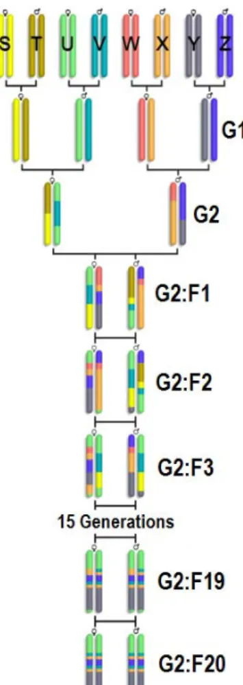
1.4 The Collaborative Cross breeding funnel (courtesy of Prof. Leonard Mcmillan). S, T, U, V, W, X, Y, and Z denote the 8 founders. The breeding funnel consists of 2 generations of crosses (G1 and G2), followed by 20 generations of inbreeding (G2:F1 - G2:F20) . . . 5

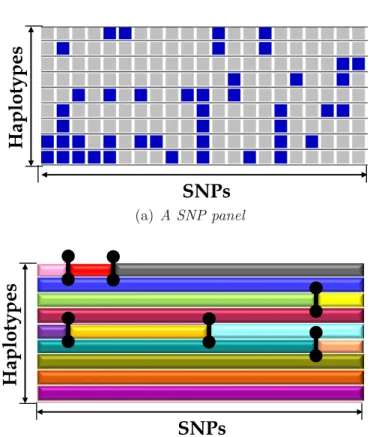
1.5 Illustration of a mosaic structure on a SNP panel. Gray and blue cells in (a) represent majority and minority alleles, respectively. The black vertical bars in (b) represent the recombination breakpoints that result in a mosaic structure. . . 9

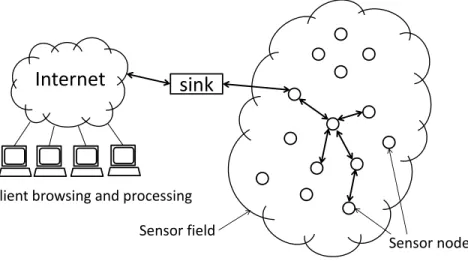
1.6 Illustration of a wireless sensor network. The edges with arrows between sensor nodes represent the routing structure. . . 11

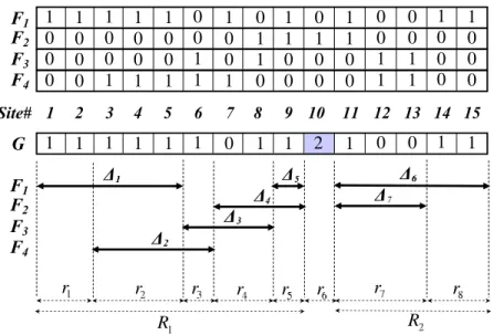
2.1 An example subregions. F1-F4 are four founder sequences. G is the

genotype sequence to be segmented. There are 15 sites in all sequences, where site 10 is the only heterozygous site. R1 : [1,9] and R2 : [11,15]

are the homozygous regions. ∆1-∆5 are the maximal shared intervals in

R1. ∆6 and ∆7 are the maximal shared intervals in R2. r1−r8 are the

subregions for the entire sequence, out of which r6 is the heterozygous

subregions, and the remaining are the homozygous subregions. . . 28

2.2 The Collaborative Cross breeding funnel. S, T, U, V, W, X, Y, and Z denote the 8 founders. The breeding funnel consists of 2 generations of crosses (G1 and G2), followed by 20 generations of inbreeding (G2:F1 -G2:F20) . . . 36

2.3 The 8 founder strains chosen for the Collaborative Cross breeding funnel shown in Fig. 2.2 . . . 37

(13)

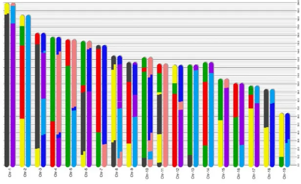
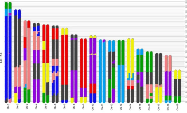
2.5 The segmentation result of the proposed algorithm on a Pre-CC animal 13m72 from Collaborative Cross. The colors of diﬀerent segments repre-sent diﬀerent founders shown in Fig. 2.3. . . 38

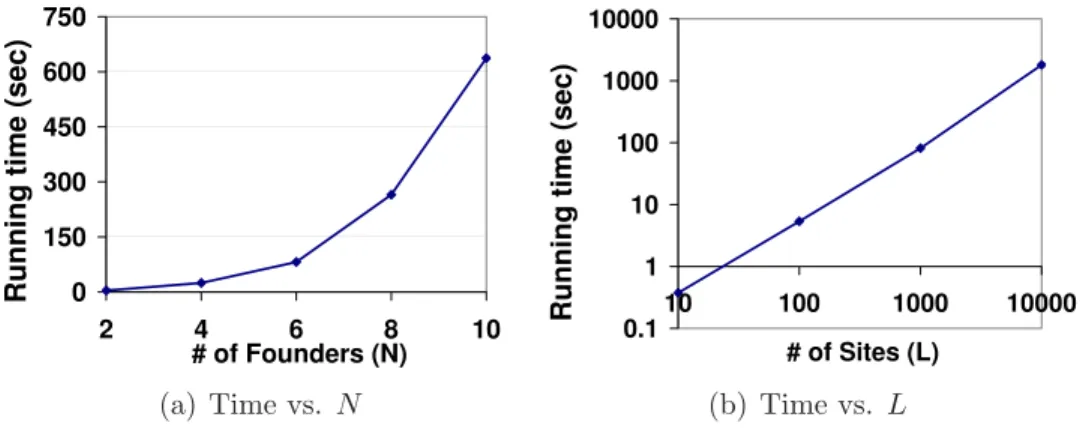
2.6 Running time with varying parameters. . . 39

2.7 Segmentation results on data with noise. . . 41

3.1 Neighboring blocks BL, BR fall inside overlapping/adjacent maximal

in-tervals IL, IR respectively. The dots in the shaded region represent

in-compatible SNP pairs ofIL and IR. . . 47

3.2 Neighboring blocks BL, BR contain diﬀerent subsets of the incompatible

SNP pairs. The dots represent the incompatible SNP pairs contained in the overlapping maximal intervalsIL and IR. The dots inside the shaded

triangle are contained in the neighboring block pair BL and BR. . . 50

3.3 Three block pairs form a node. Block pair 1, 2, and 3 are the left, middle, and right block pair of the node respectively. The breakpoint range of the node is the intersection of the end range of block pair 1, the breakpoint range of block pair 2, and the start range of block pair 3. The vertical stripes correspond to the start range, breakpoint range, and end range of a block. The marked haplotypes in the stripes are the haplotypes which have breakpoints in the corresponding region. . . 52

3.4 Comparison of Minimum Mosaic and Hapbound/SHRUB results on ADH data. (a): the Minimum Mosaic result; (b): the result inferred from the ARG in (c); (c): the ARG computed using SHRUB(Song and Hein (2005)). The bars in (a) and (b) represent the breakpoints. The dots in (c) represents the recombination events. . . 54

3.5 Comparison of the running times of MinMosaic and Hapbound over vary-ing number of SNPs (in log scale). The datasets used are from Chr19 of 51-strain dataset and 74-strain dataset. The number of SNPs included varies from 1000 to 4000. . . 56

4.1 EH summary at a site: This ﬁgure highlights the multi-level structure of EH-summary. The incoming data is buﬀered in equi-sized blocks B1,

B2,. . . ,Bj, . . ., each of size O(_εkd). The coreset C

1

j is computed for each

block Bj and sent to level l = 1. At each level l > 0, whenever two

coresets Cjl, C l

j+1 come in, they are merged and another coreset C l+1 (j+1)/2

on Cjl

Cj+1l is computed and sent to level l + 1. There are at most

log_k/εNd levels. . . 67

(14)

4.2 Error accumulation of Height-aware and Path-aware algorithms. This ﬁg-ure compares the diﬀerent strategies of assigning additive approximation factors at each site of the tree for height-aware and path-aware algorithms. Height-aware algorithm assigns the additive error uniformly to _2hε, where

h is the height of the tree. Path-aware algorithm assigns the additive error uniformly inside each sub-path, but diﬀerently for diﬀerent sub-paths. 75

4.3 Performance of the algorithms as a function of the total stream size: The overall communications among the sensor network nodes perform k-median clustering are measured using real and synthetic data. The NYSE data consists up to 28K records and the synthetic data consists up to 9 million data values. The approximation error threshold is set to 0.05. For real data, all three algorithms are tested on a 5-node system. For synthetic data, the algorithms are tested on a 10-node system. Figs. 4.3(a) and 4.3(b) demonstrate the overall data communication of the algorithms as a function of input data size. Figs. 4.3(c) and 4.3(d) demonstrate the max per node data communication of the algorithms as a function of input data size. The experiments demonstrate a signiﬁcant reduction in the overall and max per node communication. . . 80

4.4 Performance of the algorithms as a function of the number of sites. The data communication of the algorithms is measured as a function of the number of sites on NYSE and synthetic data. . . 81

4.5 Performance of the algorithms as a function of approximation error: The overall communication of the algorithm decreases as the error increases. Figs. 4.5(a) and 4.5(b) highlight the overall data communication as the error increases. Figs. 4.5(c) and 4.5(d) demonstrate the max per node data communication as the error increases. Approximate clustering is performed on NYSE data with 30K data records and synthetic data with 5 million observations. As the error tolerance increases, it can be ob-served that both the height-aware and path-aware algorithms perform better than the topology-oblivious algorithm and can further reduce the communication by additional 10−30%.. . . 82

5.1 Multi-level summary S: This ﬁgure highlights the multi-level structure of the -summary S = {s0, s1, . . . , sL}. The incoming data is divided

into equi-sized blocks of size b and blocks are grouped into disjoint bags,

B0, B1, . . . , Bl, . . . , BL with Bl for level l. B0 contains the most recent

block, B1 contains the older two blocks, and BL consists of the oldest 2L

blocks. At each level, sl is maintained as the l-summary for Bl. The

(15)

5.2 Sorted Data: The sorted and reverse sorted input data are used to mea-sure the best possible performance of the summary construction time us-ing the algorithm and GK01. Fig. 5.2(a) shows the computational time as a function of the stream size on a log-scale for a fixed epsilon of 0.001. It is observed that the sorted and reverse sorted computation time curves for GK01 are almost overlapping due to the log-scale presentation and small difference between them (average 1.16% difference). Same reason for the sorted and reverse sorted curves for the algorithm, and the average difference between them is 2.1%. It is also observed that the performance of the algorithm is almost linear and the computational performance is almost two orders of magnitude faster than GK01. Fig. 5.2(b) shows the computational time as a function of the error. It is observed that the higher performance of the algorithm which is 60−300× faster than GK01. Moreover, GK01 has a significant performance overhead as the error becomes smaller. . . 97

5.3 Random Data: The random input data is used to measure the perfor-mance of the summary construction time using the algorithm and GK01. Fig. 5.3(a) shows the computational time as a function of the stream size on a log-scale for a ﬁxed epsilon of 0.001. It is observed that the perfor-mance of the algorithm is almost linear. Furthermore, the log-scale plot indicates that the algorithm is almost two orders of magnitude faster than GK01. Fig. 5.3(b) shows the computational time as a function of the er-ror. It is observed that the algorithm is almost constant whereas GK01 has a signiﬁcant performance overhead as the error becomes smaller. . . 98

5.4 Sorted Data: The sorted and reverse sorted input data are used to mea-sure the best possible performance of the summary construction time us-ing our biased quantile algorithm and uniform quantile algorithms ZW07, GK01 using the same error 0.001. This log-scale plot indicates that our algorithm achieves up to 75x higher performance compared to GK01 and comparable performance to ZW07. Fig. 5.4(b) indicates the performance of the our biased quantile algorithm and the uniform quantile algorithms on a 10M stream size. . . 113

5.5 Random Data: The performance of the summary construction time using our biased quantile algorithm and GK01 over random data. Fig. 5.5(a) shows the computational time as a function of the stream size on a log-scale for a ﬁxed epsilon of 0.001. It is observed that our algorithm is able to compute 1.4-1.6M quantiles per second. In practice, our algorithm is over 30x faster than prior biased quantile algorithms. . . 115

(16)

Chapter 1 Introduction

The recent proliferation of high throughput technologies has catalyzed the transforma-tion of traditransforma-tional science to data-driven science. The unprecedented growth of scientiﬁc datasets leads to the phenomenon of data rich but information poor, demanding for rev-olutionary knowledge discovery techniques to assist and accelerate scientiﬁc discovery.

In this thesis, I present explorative and descriptive modeling with efficient data mining algorithm design for knowledge discovery on two types of emerging large-scale sequence-based scientific datasets: 1) static sequence data generated from SNP diversity arrays for genomic studies, and 2) dynamic sequence data collected in a streaming and sensor network for environmental studies. Both types of datasets are large-scale, containing hundreds of millions of observations. Mining useful patterns, trends, and even anomalies from these datasets can provide valuable insights to the scientific discoveries. The massive, noisy, or distributive, online nature of many datasets poses challenging issues for mining algorithm design such as scalability, robustness, and efficiency.

1.1 Mining Genomic Data

(17)

high-quality draft of the mouse genome was produced and analyzed in 2002 by the Mouse Genome Sequencing Consortium. The amount of whole-genome data is growing at an unprecedented rate, with over 1000 whole-genome datasets currently completed or under construction. This new wealth of information is quickly outstripping our ability for analysis in genetic studies, such as recombination detection and association mapping.

1.1.1 Genome-Wide SNP Arrays

Genetic variation plays an important role in determining people’s disease susceptibilities and responses to drugs and vaccines. Genome-wide Single-Nucleotide Polymorphism (SNP) arrays provide a comprehensive view of genome variation and serve as powerful resources for genetic and biomedical studies.

Markers for Genetic Variation – SNP

The genetic information of a living organism is encoded in DNA sequences. A DNA sequence consists of the sequence of nucleotide bases (adenine (A), cytosine(C), gua-nine(G) or thymine(T)) in a DNA strand. For any two humans, 99.9% of their DNA sequences are identical. Of the remaining sites that are polymorphic between two peo-ple, 80% are single-nucleotide polymorphism (SNP) sites (Fig. 1.1), where there are at least two alleles occur in the observed population with a frequency above 1%. Genome-wide SNP arrays represent one of the most comprehensive tools for measuring genetic variation. A map of more than 3.1 million SNPs over the human genome has been generated through The International Hapmap Project. For the mouse genome, NIEHS and Perlegen Sciences have generated a genome-wide map of 8.27 million SNPs over 15 commonly used strains of inbred laboratory mice.

The sequence of SNPs on a chromosome is referred to as ahaplotype sequence. Most of the SNPs are biallelic, with only two alleles at any site across the population. The allele with higher frequency is called the majority allele, the other is called the minority

(18)

Figure 1.1: Illustration of 3 SNP sites in a panel of DNA sequences from four strains

allele. For diploid animals such as human and mouse, each chromosome has two copies, and each copy corresponds to a haplotype sequence. The combination of the alleles at a SNP site is referred to as agenotype. The current technology for obtaining the genotype sequence is called genotyping, which determines for each locus, whether the genotype is homozygous for the majority allele (both haplotypes have majority allele), homozygous for the minority allele (both haplotypes have minority allele), or heterozygous (the two haplotypes have diﬀerent alleles).

Sources of Genetic Variation – Recombination and Mutation

The two major molecular events shaping genetic variation current populations are re-combination and mutation.

• Recombination

During meiosis in sexual organisms, two homologous chromosomes cross over and exchange genetic material (Fig. 1.2). Recombination leads to oﬀsprings with diﬀerent combinations of genetic variants from their parents.

• Mutation

(19)

Figure 1.2: Recombination event during meiosis

Figure 1.3: Point mutation (base “C” changed to “A”)

1.1.2 Inferring Genetic Variation Patterns

Patterns of genetic variation in a population are the product of mutation and recom-bination events that have occurred over many generations from the ancestors of the population. Understanding genetic variation patterns plays an important role in solving many genetic problems such as reconstructing genealogies and gene association studies.

Inferring Segmentation Structure of a Single Recombinant Strain

Current animal resources for genetics research are often derived by mating a small set of founders. The meiotic recombination events during the mating in each generation result in a fragmental structure in the derived recombinant strains. During the process of generating these model organisms, mutations rarely happen and are considered as

(20)

Figure 1.4: The Collaborative Cross breeding funnel (courtesy of Prof. Leonard Mcmil-lan). S, T, U, V, W, X, Y, and Z denote the 8 founders. The breeding funnel consists of 2 generations of crosses (G1 and G2), followed by 20 generations of inbreeding (G2:F1 - G2:F20)

noise.

(21)

nearly 90% of the known variation in laboratory mice, providing unparalleled power for disease association studies. As shown in Fig. 2.2, the CC strains (G2:F20) and the pre-CC strains (G2:F1-G2:F19) are composed of segments from the 8 founder sequences. The segmentation structure identiﬁes the ancestral origin of each region on a recombinant strain, which is important input for subsequent association studies.

In this thesis, I investigate the problem of inferring the segmentation structure for the recombinant strains given a small set of founder sequences. The challenges for solving this problem are three fold:

• Genotype input

Compared with DNA sequence, genotypes are less expensive to obtain experi-mentally. Algorithms with genotype input are thus more desirable. However, for genotype sequence, the exact allele combinations at heterozygous sites cannot be directly derived. To infer the two plausible haplotypes given the genotypes, phasing algorithms are usually applied, which are known to be computationally intensive.

• Biological constraints

Biologically relevant constraints are critical in defining the biologically feasible solutions for the segmentation problem. For example, in the Collaborative Cross, a specific breeding scheme (the order of the 8 founder strains coming into the funnel) defines the set of possible founder pairs for the genotype at each locus. Moreover, since each autosome undergoes one recombination event on average during each meiosis, the number of segments on the two associated haplotypes of the genotype is expected to be comparable. Without considering these biological constraints, the algorithm may generate spurious solutions.

• Noise in the data

(22)

Noise is common in biological datasets. There are both biological and technical sources of noise in genotyping, which include point mutations, gene conversions, and genotyping errors. In addition, there may be missing values in the data. Noise and missing values need to be properly modeled to make the algorithm robust for running on real biological datasets.

Previous studies have focused on similar but diﬀerent models.

• Combinatorial analysis of founder set reconstruction problem

In (Ukkonen (2002)) and (Wu and Gusﬁeld(2007)), combinatorial approaches are employed to solve the founder set reconstruction problem with a given set of sample haplotype sequences that are evolved from a small set of founders. Diﬀerent from these models, I study the “inverse” problem where the set of founder sequences are already known, and compute the segmentation structure for genotype sequences of the recombinant strains given the founder sequences. The problem is important for analyzing the ancestral polymorphism presented in experimental model resources for subsequent gene association studies. A real motivating study is analyzing the segmentation structure for pre-CC strains in Collaborative Cross.

• Probabilistic inference of SNP origin

Mott (Mott et al. (2000)) et al. proposed an HMM-based algorithm for inferring the probability of each founder pair as the origin for each genotype at a SNP site, assuming the founder sequences are known beforehand. Diﬀerent from the HMM-based algorithm, I study the problem of explicitly deriving all the possible segmentation structures with certain biological meaningful optimization criterion.

• Other related problems

(23)

(2002);Schwartz et al. (2003)), computing phylogenies (Gusﬁeld (2002); Gusﬁeld et al. (2004)).

Inferring Mosaic Structure of a Recombinant Strain Panel

Genetic recombination is an important process in shaping the arrangement of polymor-phisms within populations. “Recombination breakpoints” in a given set of genomes of a population disrupt the linkage disequilibrium (LD) existing in the genomes and divide the genomes into haplotype blocks, resulting in a mosaic structure (Fig. 1.5). Without prior knowledge of the founder sequences, this mosaic structure can only be inferred through the estimation of recombination breakpoints. Recombination breakpoints rep-resent the locations where the crossovers have occurred, either during the generation of the haplotype itself, or in previous generations (carried over from ancestors).

Under the inﬁnite site model (which assumes at most 1 mutation at each site), the recombination breakpoint can be inferred using the Four Gamete Test (FGT). The FGT states that the number of diﬀerent allele combinations between any two sites can at most be 3 if no visible recombinations have happened in between. Two SNPs are called incompatible if all 4 allele combinations exist. In this thesis, I investigate the problem of inferring the genome-wide mosaic structure consisting of the set of the recombination breakpoints which explain the SNP incompatibilities using FGT.

The challenges of inferring the genome-wide mosaic structure comes from the sheer scale of the data. For a SNP panel of tens of strains over hundreds of thousands of SNPs (a typical size for a mouse chromosome), the number of possible sets of recombi-nation breakpoints would grow exponentially in the size of the panel. Solving large-scale combinatorial problem requires eﬃcient algorithm design.

Many algorithms have been developed for several related problems, such as esti-mation of recombination rate (Hudson and Kaplan (1985); Myers and Griﬃths (2003);

Song et al.(2005)), inferring haplotype block structure (Gabriel et al.(2002);Patil et al.

(24)

(a) A SNP panel

(b) The mosaic structure on the SNP panel in (a) result-ing from historical recombinations

Figure 1.5: Illustration of a mosaic structure on a SNP panel. Gray and blue cells in (a) represent majority and minority alleles, respectively. The black vertical bars in (b) represent the recombination breakpoints that result in a mosaic structure.

(2001)), recombination detection (Posada (2002); G.F. (1998);Hein (1990, 1993); N.C. and Holmes(1997);Holmes et al.(1999);Lole et al. (1999);Martin and Rybicki (2000);

Drouin et al.(1999);Jakobsen et al.(1997);Maynard and Smith(1998);Stephens(1985);

(25)

1.2 Mining Environmental and Ecological Data

With recent advances in sensor technology, large-scale wireless sensor networks are de-ployed for observing the natural environments, monitoring habitat and wild popula-tions, offering environmental and ecology scientists access to enormous volumes of data collected from physically-dispersed locations in a continuous fashion. Some of the ex-perimental systems deployed include Berkeley’s habitat modeling at Great Duck Island (Szewczyk et al. (2004)), FLOODNET project1 which provides a flood warning in the UK, and SECOAS project2 which monitors coastal erosion around small islands in-tended as wind-farms. The large-scale, distributive and online nature of sensor network and stream data presents new computational challenges for data mining tasks such as mining the distribution of the data, mining frequent patterns or temporally drifting, evolving, periodic patterns, and anomaly detection. Adding to the challenges are strin-gent system constraints including limited size of memory, battery, and processing power of the sensor nodes. In this thesis, I investigate several related problems to discover the data distribution online for sensor network and stream systems. These problems in-clude clustering analysis and order-statistics computation, which is critical for real-time monitoring, anomaly detection, and domain specific analysis.

1.2.1 Streaming and Sensor Data

The recent advances in sensor technologies enables environmental and ecological data collection at an unprecedent scale and rate. A wireless sensor network is composed of spatially distributed sensors which are battery-powered mini computers that can monitor the environmental measurements such as temperature, sound, light, pressure, motion or pollutants at diﬀerent locations (Fig. 1.6). A typical sensor node includes

1_{http://envisense.org/ﬂoodnet.htm}

2_{http://envisense.org/secoas.htm}

(26)

an antenna and a radio frequency (RF) transceiver to allow communication between sensors, a CPU, a memory unit, a power source such as battery, and a sensor unit which collects environmental measurements.

Figure 1.6: Illustration of a wireless sensor network. The edges with arrows between sensor nodes represent the routing structure.

Sensors communicate with each other using multi-hop connections. The data is transmitted towards a special kind of node called a base station (or sink). A base station links the sensor network to the Internet for further browsing and processing at the client side. Base stations usually have enhanced capabilities over the sensor nodes to provide more complex data analysis.

Streaming sensor data and its characteristics

Observations and measurements are collected at each sensor node continuously as data streams – the ordered sequence of sensor readings. Diﬀerent from static datasets, data streams present several unique characteristics:

• Data streams are real-time, and possibly high-speed.

(27)

• Data streams are potentially unbounded in size.

Once deployed, the sensors continuously collect the measurements which result in massive amount of data over time.

• Data streams cannot be explicitly stored.

Due to the limited memory at each sensor, the massive-scale of raw readings in data streams cannot be completely stored for further retrieval and processing.

Additionally, for sensor network systems,

• Multiple data streams are collected in a distributed fashion.

The distributed data streams are organized according to the routing topology of the sensor network. The data are eventually collected at the sink.

1.2.2 Challenges with Mining Streaming and Sensor Data

The unique characteristics of streaming and sensor network data lead to a number of computational and data mining challenges:

• The sheer volume of the data streams and the limited memory make it impossible

to store the entire data stream or even scan the data multiple times. The data mining algorithms are thus required to be single pass, or a few passes.

• The continuous, real-time nature of the data streams requires data mining

algo-rithms to be continuous, incremental, and on-the-ﬂy.

In addition, the system constraints of sensor network pose extra computational chal-lenges for data mining algorithm design:

• Sensor nodes are inherently resource-constrainted. They have limited storage

ca-pacity, battery, and processing power. The sensors are sometimes deployed in

(28)

hazardous environment which are inaccessible after deployment. The major drain on the sensor’s battery is data transmission, which determines the lifetime of the sensor node. Therefore, the data mining algorithms are required to be resource-aware.

• The wireless sensor networks are essentially distributed data stream systems. Due

to the limited power, it is not aﬀordable to transmit all local streams of raw sensor readings towards the sinks for centralized processing. As a result, the data mining algorithms need to be distributed across the sensor nodes.

1.2.3 Capturing Data Distribution - Clustering and Order

Statis-tics Computation

In this thesis, I present several algorithms to discover the data distribution online and continuously for streaming and sensor network systems including clustering analysis and order-statistics computation.

Clustering Distributed Data Streams

Clustering, a useful tool in data analysis, is the problem of ﬁnding a partition of a dataset so that, under a given distance metric, similar items are grouped together. Clustering the data collected in distributed data streams systems such as a sensor network provides a good estimation of the underlying data distribution.

Clustering over distributed streams is a challenging task. Diﬃculties lie in various issues:

• Communication

(29)

one of the techniques (Olston et al. (2003);Madden et al.(2002);Silberstein et al.

(2006);Willett et al.(2004)) that push processing operators down into the network to reduce data transmission. It computes a local summary at each site and merges and summarizes further at each internal site towards the root. However, this approach cannot be immediately adopted to solve the clustering problem, since clustering is usually a holistic computation (Madden et al. (2002)) which cannot be readily decomposed into computations on data partitions.

• Clustering Quality

Accuracy is usually traded for reduced communication through sketching or syn-opsis construction. However, it is necessary to provide approximate distributed clustering with a guaranteed bounded error.

• Topology

The topology of the underlying routing network is an important factor that in-ﬂuences the performance of the distributed clustering algorithm. The topology sensitivity of the algorithm determines the adaptability of the algorithm given diﬀerent knowledge about the routing topology.

Order Statistics Computation on High-Speed Data Streams

In addition to clustering analysis, order statistics is also one of the fundamental tools to capture the distribution of the dataset, by associating the rank and value of the data. As a popular order statistics, quantiles have found wide application in database and scientific computing. Different from quantile computation on static datasets, streaming quantile computation is required to be single-pass, space efficient and continuous.

Many algorithms have been proposed for computing approximate quantiles over the entire stream history (Manku et al.(1998);Greenwald and Khanna(2001)) or over a slid-ing window (Lin et al. (2004); Arasu and Manku (2004)); with uniform error (Manku

(30)

et al. (1998); Greenwald and Khanna (2001)) or with biased error (Cormode et al.

(2005, 2006)). The best reported storage bound for approximate quantile computation is O(1/log(N)) (Greenwald and Khanna (2001)), where N is the size of the stream, andis the approximation bound. However, most of these algorithms focus on reducing the space requirement at the expense of the computational cost, which is important for processing high-speed data streams with satisfactory real-time performance. In addi-tion to single-pass and continuous computaaddi-tion, the requirements for eﬃcient quantile computation algorithms over high-speed data streams are:

• The algorithm should have a lowe per element computation cost as well as low

storage bound.

• In order to guarantee the precision of the result, the algorithm should ensure

random or deterministic error bound for the quantile computation.

• The algorithm should be able to handle stream size which is not known a priori.

1.3 Thesis Statement

Eﬃcient algorithms can be designed for mining massive sequence-based scientiﬁc datasets from emerging biological and environmental applications such as genomic datasets and streaming and sensor datasets using block-based decomposition methods.

1.4 New Results

(31)

1.4.1 Mining Genome Data

Inferring Segmentation Structure of a Single Recombinant Strain

• ModelI propose the Minimum Segmentation Model to infer the origins of haplo-type segments in a recombinant strain (genohaplo-type sequence) given a set of known founders (haplotype sequences). Each segment on a recombinant strain is at-tributable to one of the founders. The minimum segmentation can be used for inferring the relationship among recombinant sequences to identify the genetic ba-sis of traits, which is important for disease association studies. The basic model is also extended to handle noise and support additional biologically-motivated con-straints. The biological constraints include the funnel breeding scheme and the requirement of comparable number of segments on both haplotypes. These con-straints guarantee the biological validity of the solutions as well as signiﬁcantly reduce the search space. Furthermore, noise (point mutations, gene conversions, and genotyping errors) and missing values, as common to all biological datasets, are incorporated to improve the robustness of the model.

• AlgorithmI propose eﬃcient dynamic programming algorithm to solve the Min-imum Segmentation problem in polynomial time based on block-wise decomposi-tion of the sequences. The algorithm has a time complexity of O(LN +P4) and a space complexity ofO(P N2_{), where} _L_{is the number of SNPs,} _N _{is the number}

of founders, and P is the number of blocks.

• Performance The proposed algorithms permits genome wide analysis on real mouse genome datasets (Collaborative Cross), and generates feasible biological solutions on CC (preCC and G2F1 strains). The proposed algorithm can also handle noise and missing values properly on these strains.

(32)

Inferring Mosaic Structure of a Recombinant Strain Panel

• Model I propose the Minimum Mosaic Model to capture the minimum number of recombination breakpoints required for generating a set of genome sequences (in haplotypes). This mosaic structure provides a good estimation of the rate and possible locations of the recombination events, which is useful for inferring haplotype block structures and genealogical history.

• AlgorithmI proposed an eﬃcient graph-based algorithm for computing the min-imum mosaic structure for a given set of haplotype sequences. The strains in the SNP arrays are divided into blocks. For any two neighboring haplotype blocks, the local breakpoints are inferred according to the Four-Gamete Test (FGT). Pos-sible local breakpoint sets (as graph nodes) are connected to form a combinatorial search space for minimum solution.

• Performance The proposed algorithm permits genome-wide analysis. The ex-periments on CGD mouse genome datasets with 51 mouse strains over total 7.8M SNPs demonstrates the good performance of the algorithm (less than half an hour for each chromosome).

1.5 Mining Environmental and Ecological Data

Clustering Distributed Data Streams

• ModelI deﬁne the problem of approximate k-Median Clustering over data arriving at a distributed data stream system such as a sensor network.

(33)

data transmission between sites, which is the main drain on the sensor’s battery. Eﬃcient summary structures are designed to reduce data transmission as well as guarantee bounded-error solution. The summary structure is constructed by di-viding the in coming streams into ﬁxed-size blocks. The algorithms reduce the maximum per node transmission topolylogN (opposed to N for transmitting the raw data).

• Performance The algorithms demonstrate the scalability of the algorithms with respect to the data volume, approximation factor, and the number of sites. All three algorithms can greatly reduce the total as well as per node transmission, especially with larger-scale data.

Order Statistics Computation on High-Speed Data Streams

• ModelI solve the problem of approximate quantile and biased-quantile for high-speed data streams.

• AlgorithmI propose a fast algorithm for computing approximate quantiles in high speed data streams with deterministic error bounds. The algorithm uses simple block-wise merge and sample operations. Overall, the proposed algorithm achieves a per-element update computational cost ofO(log(1/log(N))) for approximation factor and stream size N (N is not know beforehand). In addition, I proposed an efficient algorithm for computing approximate biased quantiles in large data streams. The algorithm is based on a novel piece-wise uniform sampling technique which computes decomposable biased quantile summaries on fixed size blocks of the incoming data stream. The algorithm is computationally efficient, does not assume prior knowledge of the stream sizes or the range of data values in the streams, and is applicable to distributed data stream system. In practice, the algorithm is able to efficiently maintain summaries over large data streams with

(34)

over tens of millions of observations.

• PerformanceExperiments demonstrate that the algorithms are able to eﬃciently maintain summaries over large data streams with over tens of millions of observa-tions.

1.6 Organization

The rest of the thesis is organized as follows:

• Chapter 2presents the Minimum Segmentation model and algorithms for solving the problem of inferring segmentation structure of a single recombinant strain.

• Chapter 3 presents the Minimum Mosaic model and algorithms for solving the problem of inferring mosaic structure of a recombinant strain panel.

• Chapter 4presents the algorithms for approximate K-Median clustering for sen-sor network data.

• Chapter 5presents the algorithms for approximate quantiles and biased-quantiles computation high-speed data streams.

(35)

Chapter 2 Inferring Segmentation Structure of

Recombinant Genotype Sequences

2.1 Introduction

Recombination plays an important role in shaping the genetic variations present in current-day populations. Understanding the genetic variations and the genetic basis of traits is crucial for disease association studies. We assume an evolution model (previously proposed and studied in (Ukkonen(2002);Wu and Gusﬁeld(2007))) where a population is evolved from a small number of founder sequences. A real-world biological scenario is the Collaborative Cross (CC). The CC (Churchill et al.(2004);Threadgill et al.(2002)) is a large panel of 1000 recombinant inbred (RI) mouse strains that were generated from a funnel breeding scheme initiated with a set of 8 founder strains followed by 20 generations of inbreeding. These 8 genetically diverse founder strains capture nearly 90% of the known variations present in the laboratory mouse. The resulting RI strains have a population structure that randomizes the known genetic variation, which provide unparallel power for disease association studies.

(36)

label these segments according to their contributing founder. Although the segmenta-tion for a haplotype sequence may be straightforward to compute, in many cases the sequence to be segmented is a genotype sequence for which the two haplotypes are not completely distinct and they may have diﬀerent segmentations. For example, the mice generated during the intermediate generations in the CC funnel are genotyped to obtain the genotype sequences each of which contains two diﬀerent haplotypes in each line.

I study the segmentation problem of genotype sequences with the optimization for the minimum number of segments contained in the two associated haplotypes. Furthermore, I extend this basic model to include additional biologically-motivated constraints as well as noise. Since each autosome undergoes, on average, one recombination per meiosis, it is expected that the number of founder switches per haplotype at a given generation of breeding are comparable. Moreover, noise may exist in the founder sequences as well as the genotype sequence to be segmented. Sources of the noise are both technical and biological. They include point mutations, gene conversions, genotyping errors, etc. In addition to noise, missing genotyping values are also very common in these datasets.

2.2 Related Work

Similar but diﬀerent models were studied in (Ukkonen (2002); Wu and Gusﬁeld (2007);

(37)

models, the genotype sequence segmentation problem studied in this thesis assumes that the set of founder sequences are already known, and the main focus is on inferring the segmentation structure for genotype sequences, with the consideration of biologically-relevant constraints and noise present in the data. The genotype sequence segmentation problem is very important for studying the ancestral polymorphism structure in experi-mental recombinant strains such as PreCC strains (strains from intermediate generations in the CC funnel which are not fully inbred).

Besides the combinatorial analysis of founder set reconstruction problem presented in (Ukkonen(2002)) and (Wu and Gusﬁeld(2007)), another line of related work focuses on probabilistic inference of SNP origins. Mott (Mott et al. (2000)) et al. proposed an HMM-based algorithm for inferring the probability of each founder pair as the origin for each locus, assuming the founder sequences are known beforehand. The founder origin probability distribution is computed for outbred animal stocks as input for subse-quent quantitative trait loci (QTL) mapping. Diﬀerent from locus-based founder origin estimation in (Mott et al.(2000)), the genotype sequence segmentation problem explic-itly derives all the possible segmentation structures with certain biological meaningful optimization criterion.

Other related work of analyzing the genetic variation structure of the genome se-quences include identifying haplotype blocks (Dally et al. (2001); Gabriel et al. (2002);

Schwartz et al. (2003)), computing the phylogenies (Gusﬁeld (2002); Gusﬁeld et al.

(2004)), etc.

2.3 The Minimum Segmentation Problem

Assume that we have a set of founding haplotypes F S = {F1, . . . , Fn, . . . , FN}. Each

haplotype sequence is of length L: Fn = fn

1f

n l . . . f

n

L, where f n

l ∈ {0,1}. Given an input sequence from a population which is derived exclusively from the founder set F S,

(38)

the problem is to ﬁnd a possible segmentation of the sequence, where each segment is inherited from the corresponding region of one of the founders. I ﬁrst explain the simple case where the input sequence is a haplotype, and then investigate the more interesting case where the input is a genotype sequence.

Given a haplotype sequence, H =h1. . . hL, (hl ∈ {0,1}), a segment of H is denoted

asHk =hs_khs_k+1hs_k+L_k−1, where sk is the starting position ofHk, and Lk is the length

of Hk. A segmentation of H divides the entire sequence into an ordered list of disjoint segments Seg(H) = {H1, . . . , Hk, . . . , HK}, where each segment Hk is identical to the

corresponding region of one of the founders andK is the number of segments inSeg(H). In other words, for each segment Hk = hs_khs_k+1hs_k+L_k−1, there exists a founder Fn =

f1nf

n l . . . f

n

L such thathsk+li =f n

s_k+l_i, for li = 0,1, . . . , Lk−1. Furthermore, a minimum segmentation is deﬁned as the segmentation which contains the minimum number of segments. The minimum segmentation is denoted as M inSeg(H) ={H1, . . . , HK_min},

where Kmin =|M inSeg(H)| is the number of segments in M inSeg(H).

If the input is a genotype sequence, it represents two copies of diﬀerent haplotype sequences, Ha and Hb. Assume that the genotype sequence is G = g1. . . gL, where

gl ∈ {0,1,2}. A site l is homozygous if gl = 0 (hal = h b

l = 0) or gl = 1 (h a l = hbl = 1); a site l is heterozygous if Ha and Hb take diﬀerent alleles, in which case, gl = 2. The process of determining whether ha

l = 0, h b

l = 1 or h a

l = 1, h b

l = 0 for a heterozygous site l is called phasing. The procedure of determining the two haplotype sequences from the genotype sequence by phasing all the heterozygous sites is called

Haplotype Inference. For the genotype input case, a segmentation Seg(G) consists of segmentations for both haplotype sequences: Sega(Ha) and Segb(Hb). The number of segments in Seg(G) is the sum of the numbers of segments inSega(Ha) and Segb(Hb): |Seg(G)| = |Sega(Ha)|+|Segb(Hb)|. The minimum segmentation is the segmentation

(39)

I develop eﬃcient algorithms for the minimum segmentation problem especially for the genotype input case. In addition to the basic models, there are other issues which need to be considered, such as genotyping errors, point mutations, missing values, the balance of the number of segments in both haplotypes, etc. I will explain later how these biological constraints and noise are modeled in the solutions.

Solutions for Haplotype Input: Computing the minimum segmentation for the haplotype input sequence is relatively easy and has been discussed in previous studies (Wu and Gusﬁeld (2007); Ukkonen (2002)). A simple greedy algorithm can be applied to compute a minimum segmentation solution by scanning from left to right. Assume that the current site is i (initially it is site 1), and we have a minimum segmentation solution for the part of the input sequence from site 1 to site i. Starting from site i, we try to ﬁnd the segment shared by the input sequence and one of the founders which extends furthest to the right. This greedy algorithm generates one of the minimum segmentation solutions.

A graph-based dynamic programming algorithm can be used to compute all minimum segmentation solutions given the input haplotype sequence and the founder set. At a high level, all maximal shared intervals are ﬁrst computed between the input sequence and each founder sequence. The maximal shared interval between the input sequence and founder n is a region where the input sequence is exactly the same as founder n. Each shared interval is considered as a node and two intervals are connected with an edge if they overlap. In this way, a minimum segmentation solution corresponds to a shortest path from a node starting at the ﬁrst site to a node ending at the last site. The complete set of the shortest paths can be computed, which are all possible minimum segmentation solutions.

(40)

2.4 Solutions for Genotype Input

The greedy algorithm and the graph-based algorithm for segmenting haplotype input sequences cannot be easily applied on genotype input. The major issue is that the exact sequences of the two haplotypes are not known due to the multiple possible allele pairs at heterozygous sites. Second, the minimum segmentation solution for the genotype may not consist of the minimum segmentation solutions for each haplotype sequence.

In the following discussion, I describe two dynamic programming algorithms for solving the minimum segmentation problem for genotype input sequences. The ﬁrst algorithm considers each site separately, the second algorithm considers a region of sites simultaneously, and is thus more eﬃcient.

Site-based Dynamic Programming Algorithm: For each sitel, the possible founders for the two haplotype sequences Ha and Hb are considered. If site l is a homozy-gous site, assuming gl = 0 (without loss of generality), we have ha

l = h b

l = 0. Let ofa,l be the original founder where ha_l was inherited from at site l. Then ofa,l must be one of the founders which also take 0 at site l: ofa,l ∈ {Fn|fln = 0}. Similarly, we have the founder where hbl was inherited from as: of

b,l _{∈ {}

Fn|fln = 0}. Let f pl ₌ _ofa,l_{, of}b,l _{denote the possible founder pair at site} _l_{, we have the set of all} possible founder pairs as F Pl ₌ {_{f p}l|_{f p}l ∈ {Fn|_fn

l = 0} × {Fn|f n

l = 0}}. If site l is a heterozygous site where gl = 2, there are two possibilities: ha

l = 1∧ h b l = 0 or ha

l = 0∧h b

l = 1. Therefore, the possible founder pairs for heterozygous site l is F Pl = {f pl|f pl ∈ {Fn|f_ln = 0} × {Fn|f_ln = 1} ∪ {Fn|f_ln = 1} × {Fn|f_ln = 0}}. The founder pair setF Pl is computed for each site l.

Assigning a founder pair from F Pl to each site l generates a segmentation of the input genotype sequence. The number of segments of both haplotypes (of the geno-type) are the total number of founder switches between founder pairs of every consec-utive sites plus 2. Consider two neighboring sites l and l + 1. If the corresponding founder pairs are f pl

q_l = of a,l q_l , of

b,l

q_l (1 ≤ ql ≤ |F P

l|_{) and} _{f p}l+1

q_l+1 = of a,l q_l+1, of

(41)

(1≤ ql+1 ≤ |F Pl+1|), the number of founder switches between these two founder pairs

F ounderSwitch(f plq_l, f p l+1

q_l+1) can be computed as:

F ounderSwitch(f pl_q l, f p

l+1

q_l+1) =

⎧ ⎪ ⎪ ⎪ ⎪ ⎪ ⎪ ⎪ ⎨ ⎪ ⎪ ⎪ ⎪ ⎪ ⎪ ⎪ ⎩

0 : if ofqa,l_l =ofqa,l_l+1+1∧of b,l

q_l =ofqb,l_l+1+1 1 : if ofqa,l_l =ofqa,l_l+1+1∧of

b,l

q_l =ofqb,l_l+1+1 or

ofqa,l_l =ofqa,l_l+1+1∧of b,l

q_l =ofqb,l_l+1+1 2 : if ofqa,l_l =ofqa,l_l+1+1∧of

b,l

q_l =ofqb,l_l+1+1

(2.1)

Let Kmin(g1. . . gl−1|f plq_l) be the minimum number of segments in any segmentation solution over the subsequence g1. . . gl which at site l takes the founder pair f plq_l. The minimum number of segments over the entire genotype sequence Kmin(g1. . . gL) can be

computed as:

Kmin(g1. . . gL) =minf pL

qL∈F PL{Kmin(g1. . . gL−1|f p L

q_L)} (2.2)

The main recurrence of the dynamic programming algorithm is as follows:

Kmin(g1. . . gl−1|f plq_l) = minf pl_ql−1

−1∈F Pl−1{Kmin(g1. . . gl−2|f p l−1

q_l₋1)+

F ounderSwitch(f pl_q−1 l−1, f p

l q_l)}

(2.3)

And initially,

Kmin(Φ|f p1q1) = 2,∀f p

1

q1 ∈F P

1 _(2.4)

The solutions for this dynamic programming problem can be easily computed by populating a table T of L rows where row l has at most |F Pl| _{entries. The entry} T(l, ql), 1≤ql ≤ |F Pl|_{is ﬁlled with}_Kmin₍_g

1. . . gl−1|f plq_l) during the computation. Row

(42)

1 is initialized according to Eq.(4), and row i+ 1 is computed after row i. During the computation of T(l, ql) according to Eq.(3), backtracking pointers from entry T(l, ql) to any T(l−1, ql₋1) are preserved where the minimum values are obtained. In this way,

all the minimum segmentation solutions can be obtained.

There are at mostN2_{founder pairs for each site}_l_,_i.e._,|_{F P}l| ≤_N2_,∀_l_{. Therefore, the}

populated table is of size O(LN2_{). It takes constant time to compute} _{F ounderSwitch}

(f pl q_l, f p

l+1

q_l+1), then ﬁlling out a single entry in the table takesO(N

2_{) time. Therefore, the}

computational complexity for the entire algorithm is O(LN4). The space complexity is O(LN2). For very long sequences and a small number of founders, i.e., L N4, the algorithm has linear time and space complexity in terms of the length of the input sequence. If multiple backtrack pointers are kept for each entry while populating the table, all the minimum segmentation solutions can be obtained.

Region-based Dynamic Programming Algorithm: For very long sequences, a more eﬃcient algorithm is proposed which considers a subregion of the entire sequence instead of one site at a time.

First consider the homozygous regions, which are the regions of homozygous sites between any two consecutive heterozygous sites. Within a homozygous region, both copies of the haplotype sequences are the same and the exact allele at each site can be inferred. Fig. 2.1 illustrates an example of a set of four founders (F1 −F4) and

a genotype input sequence G to be segmented. The length of each founder and the genotype sequence is 15, with 14 homozygous sites and 1 heterozygous site (site 10). The homozygous regions areR1 = [1,9] andR2 = [11,15]. For each homozygous region,

(43)

Figure 2.1: An example subregions. F1-F4 are four founder sequences. Gis the genotype

sequence to be segmented. There are 15 sites in all sequences, where site 10 is the only heterozygous site. R1 : [1,9] and R2 : [11,15] are the homozygous regions. ∆1-∆5 are

the maximal shared intervals inR1. ∆6 and ∆7 are the maximal shared intervals inR2.

r1−r8 are the subregions for the entire sequence, out of which r6 is the heterozygous

subregions, and the remaining are the homozygous subregions.

intervalIi. Since both haplotypes are the same, a maximal shared interval for haplotype Ha is also a maximal shared interval for haplotype Hb, therefore, the maximal shared interval for the homozygous regions can also be represented as ∆i : (Ii,∗, Fn). In Fig.

2.1, ∆1 −∆5 are the maximal shared intervals within region R1 for both haplotype

sequences. Each homozygous region Rj is then divided into a set of subregions using the two end points of all maximal shared intervals inside Rj. For example, in Fig. 2.1, R1 is divided into subregionsr1, r2, r3, r4, andr5. If each heterozygous site is considered

as a 1-site subregion (e.g. r6 in Fig. 2.1), together with all the subregions for the

homozygous regions,{rp}represents a complete set of subregions which cover the entire sequence (e.g., r1−r8 in Fig. 2.1).

For each homozygous subregion rp, let f prp ₌ _ofa,rp_{, of}b,rp _{be a possible founder} pair for subregion rp. The set of possible founder pairs is F Prp ₌ {_ofa,rp_{, of}b,rp| ∃∆i1 = (Ii1,∗, ofa,rp),∆i2 = (Ii2,∗, ofb,rp), where Ii1 ⊇ rp, Ii2 ⊇ rp}. For example, the

founder pair for the subregion r2 in Fig. 2.1 could be F1, F1, or F1, F2, or F2, F1,

(44)

or F2, F2. For each heterozygous subregion which is composed of a heterozygous site

l, since hla and h l

b take diﬀerent alleles, any possible founder pair should consist of a founder taking allele 1 and a founder taking allele 0. For example, in Fig. 2.1, the possible founder pairs for r6 are F1, F2, F2, F1, F2, F3, F2, F3, F2, F4, and

F4, F2.

Instead of considering each site, each subregion is considered as a unit in the dynamic programming solution. Assignf prp

q_p =of a,r_p q_p , of

b,r_p

q_p to be the founder pair for subregion rp, where 1 ≤ qp ≤ |F Prp|_{, and} _{f p}rp+1

q_p+1 = of a,rp q_p+1, of

b,rp

q_p+1 to be the founder pair for subregion rp+1, where 1 ≤ qp+1 ≤ |F Prp+1|. Similarly, the number of founder switches

between f prp q_p, f p

r_p+1

q_p+1 is counted as:

F ounderSwitch(f prqpp, f p r_p+1 q_p+1) =

⎧ ⎪ ⎪ ⎪ ⎪ ⎪ ⎪ ⎪ ⎨ ⎪ ⎪ ⎪ ⎪ ⎪ ⎪ ⎪ ⎩

0 : if ofa,rp q_p =of

a,r_p+1 q_p+1 ∧of

b,r_p q_p =of

b,r_p+1 q_p+1 1 : if ofqa,rp p =of

a,rp+1 qp+1 ∧of

b,rp qp =of

b,rp+1 qp+1

ofa,rp q_p =of

a,r_p+1 q_p+1 ∧of

b,r_p q_p =of

b,r_p+1 q_p+1 2 : if ofa,rp

q_p =of a,r_p+1 q_p+1 ∧of

b,r_p q_p =of

b,r_p+1 q_p+1

(2.5)

LetKmin(r1. . . rp−1|f p

rp

q_p) be the minimum number of segments in any segmentation solution over the subsequence covered by r1. . . rp which takes the founder pair f p

rp qp at subregion rp. The minimum number of segments over the entire genotype sequence Kmin(r1. . . rP) whererP is the last subregion can be computed as:

Kmin(r1. . . rP) =min_{f p}rP

qP∈F PrP{Kmin(r1. . . rP−1|f p r_P

q_P)} (2.6)

The main recurrence of the dynamic-programming algorithm is as follows:

Kmin(r1. . . rp−1|f p rp

qp) = minf prp_qp−1

−1∈F Pp−1{Kmin(r1. . . rp−2|f p rp−1 q_p₋1)+

F ounderSwitch(f prp−1 q_p₋1, f p

r_p q_p)}

(2.7)

And initially,

Kmin(Φ|f prq11) = 2,∀f p r1 q1 ∈F P

Mining emerging massive scientific sequence data using block-wise decomposition methods

Mining Emerging Massive Scientiﬁc Sequence Data

using Block-wise Decomposition Methods

Abstract

Acknowledgements

Table of Contents

List of Tables

List of Figures

Chapter 1

Introduction

1.1

Mining Genomic Data

1.1.1

Genome-Wide SNP Arrays

1.1.2

Inferring Genetic Variation Patterns

1.2

Mining Environmental and Ecological Data

1.2.1

Streaming and Sensor Data

1.2.2

Challenges with Mining Streaming and Sensor Data

1.2.3

Capturing Data Distribution - Clustering and Order

Statis-tics Computation

1.3

Thesis Statement

1.4

New Results

1.4.1

Mining Genome Data

1.5

Mining Environmental and Ecological Data

1.6

Organization

Chapter 2

Inferring Segmentation Structure of

Recombinant Genotype Sequences

2.1

Introduction

2.2

Related Work

2.3

The Minimum Segmentation Problem

2.4

Solutions for Genotype Input