Second order growth model for longitudinal item response data

(1)

A Second-Order Growth Model for Longitudinal Item

Response Data

Daniel Serrano

A Dissertation submitted to the faculty of the University of North Carolina at Chapel Hill in partial fulfillment of the requirements for the degree of Doctor of Philosophy in the Department of Psychology: L.L. Thurstone Psychometric Laboratory.

Chapel Hill 2010

Approved by

Patrick J. Curran, Ph.D. Robert C. MacCallum, Ph.D.

David Thissen, Ph.D. Daniel J. Bauer, Ph.D.

(2)

c

2010

(3)

ABSTRACT

Daniel Serrano: A Second-Order Growth Model for Longitudinal Item Response Data (Under the direction of Patrick J. Curran)

This Dissertation explores the unique issues related to specifying and fitting a

second-order growth model to longitudinal item response data. The model examined is a hybrid

of the logistic IRT model for binary item responses and the latent growth curve model

for repeated measures. Attention centered around parameterization, identification,

es-timation, and issues related to estimation of the model such as convergence, improper

solutions, bias and root mean squared error (RMSE). Two variations on the proposed

model: one with correlated errors (model 2) and one without (model 1). In each model

two types of estimator were examined: full and limited information estimators. Two

sample size conditions were examined, one withN = 750 observations, and another with

N = 3000. In addition, two item parameter sets were examined, one having a wide range

of difficulty and the other, narrow. Comparing analyses stratified across model, findings

indicated greater rates of improper solutions and bias for model 2 versus model 1.

Lim-ited information estimators of model 1 performed worse than full information estimators,

while the opposite was true for model 2. Bias and convergence issues were greatest when

difficulty had a wide range. Lastly, sample size appeared to play a negligible role in bias

and RMSE, though it did affect convergence issues and improper solutions. Based on

empirical results presented in this simulation the proposed model appears to be a logical

(4)

ACKNOWLEDGEMENTS

I would like to thank my advisor, Patrick J. Curran, without whose guidance and keen

insights none of this would have been possible. I would like to thank my committee

mem-bers, who have aided this project through feedback throughout the process. Many thanks

are due to Taehun Lee, whose friendship and interest in discussing this project greatly

contributed to the successful completion. Lastly, I would like to thank the institution

of the L. L. Thurstone Psychometric Lab for providing the education, environment, and

(5)

CHAPTER

1 Introduction . . . 1

1.1 Proposed Model . . . 5

1.1.1 A Model for Correlated θ . . . 6

1.1.2 Advantages of this Approach . . . 7

1.1.3 Identification . . . 8

1.1.4 Measurement Invariance . . . 9

1.1.5 A Model For Correlated Errors . . . 10

1.2 Estimation . . . 11

1.2.1 Limited Information Estimation . . . 12

1.2.2 Full Information Estimation . . . 16

1.3 Hypotheses . . . 21

1.3.1 Model Complexity Hypothesis . . . 21

1.3.2 Estimator Hypothesis . . . 21

1.3.3 Difficulty Range Hypothesis . . . 22

1.3.4 Sample Size Hypotheses . . . 22

1.3.5 Sample Size By Estimator Hypothesis . . . 22

2 Method . . . 24

2.0.6 Model Complexity Manipulation . . . 24

(6)

2.0.8 Difficulty Range Manipulation . . . 26

2.0.9 Implied Moments . . . 38

2.0.10 Sample Size Manipulation . . . 38

2.0.11 Non-Convergence . . . 39

2.0.12 Improper Solutions . . . 39

3 Results . . . 40

3.1 Model 1 . . . 41

3.1.1 Convergence . . . 41

3.1.2 NPD Solutions . . . 41

3.1.3 First Parameter Set Bias . . . 42

3.1.4 First Parameter Set Meta Model Results . . . 44

3.1.5 Second Parameter Set Bias . . . 51

3.1.6 Second Parameter Set Meta Model Results . . . 53

3.1.7 RMSE . . . 59

3.1.8 Summary of Findings . . . 59

3.2 Model 2 . . . 60

3.2.1 Convergence . . . 61

3.2.2 NPD Solutions . . . 61

3.2.3 First Parameter Set Bias . . . 63

3.2.4 First Parameter Set Meta Model Results . . . 67

3.2.5 Second Parameter Set Bias . . . 71

3.2.6 Second Parameter Set Meta Model Results . . . 74

3.2.7 Summary of Findings . . . 78

3.3 Additional Analyses . . . 81

3.3.1 Model 1 with MCEM . . . 81

3.3.2 NPD Sensitivity Analyses . . . 82

4 Discussion . . . 85

(7)

4.2 Sample Size Effect . . . 86

4.3 Estimator Effects . . . 87

4.4 WLSMV Bias and Contingency Table Sparseness . . . 88

4.5 Recommendations for Application . . . 89

4.6 Limitations and Future Directions . . . 90

4.7 Conclusion . . . 93

5 Appendices . . . 95

5.1 Appendix 1: Parameter set 1 RMSE . . . 95

5.2 Appendix 2: Parameter set 2 RMSE . . . 99

5.3 Appendix 3: Cell Means . . . 103

(8)

LIST OF TABLES

2.1 Population Values for Item and Structural Parameters . . . 26

3.1 Experimental Design . . . 41

3.2 Item and Structural Parameter Bias for Model 1, Set 1, N=750 . . . 43

3.4 Meta Model Results: ˆa Raw Bias for Model 1, Set 1 . . . 46

3.5 Meta Model Results: ˆb Raw Bias for Model 1, Set 1 . . . 47

3.6 Meta Model Results: Fixed Effect Raw Bias for Model 1, Set 1 . . . 48

3.7 Meta Model Results: Random Effect Variance Estimate Raw Bias for Model 1, Set 1 . . . 49

3.8 Meta Model Results: Random Effect Covariance Estimate Raw Bias for Model 1, Set 1 . . . 50

3.9 Meta Model Results: ˆψ Raw Bias for Model 1, Set 1 . . . 51

(9)

3.26 Meta Model Results: ˆρ Raw Bias for Model 2, Set 1 . . . 70

3.35 Meta Model Results: ˆρ Raw Bias for Model 2, Set 2 . . . 78

3.36 MCEM Item and Structural Parameter Bias for Model 1, Set 1, N=750 . . . 81

5.1 Item and Structural Parameter RMSE for Model 1, Set 1, N=750 . . . 95

5.3 Item and Structural Parameter RMSE for Model 2, Set 1 . . . 98

5.6 Item and Structural Parameter RMSE for Model 2, Set 2 . . . 102

5.7 Item and Structural Parameter Bias Cell Means for Model 1, Set 1 . . . 104

5.8 Item and Structural Parameter Bias Cell Means for Model 1, Set 2 . . . 105

(10)

(11)

LIST OF FIGURES

2.1 ICCs for Parameter Set 1 at Time 1 . . . 30

(12)

CHAPTER 1

Introduction

Over the past 30 years psychological research has gradually shifted away from cross

sectional designs and toward longitudinal or repeated sampling designs, under which

scales are repeatedly administered to a sample of subjects tracked over multiple

assess-ment occasions. The field’s origins in experiassess-mental research likely account for the heavy

reliance on cross sectional designs. However, as research began to focus on

developmen-tal processes of both normative and pathological behavior, longitudinal designs became

prominent (Nesselroade & Baltes, 1979). Advances in statistical theory and computing

have facilitated the adoption of this approach within the field (Bollen & Curran, 2006;

Mehta & West, 2000). However, it is rare for such studies to incorporate measurement

models to account for the measurement error inherent in the study of such unobservable

psychological constructs as internalizing or externalizing behavior.

In the case of most measurement studies, single stage sampling is employed and

re-sults in the random sampling of respondents and their responses to a scale composed

of k items. This historical design resulted in the development of many useful statistical

models for assessing measurement properties in cross section, but renders the analysis of

longitudinal responses complex. The primary obstacle to specification of a latent variable

model characterizing the measurement properties of the sampled responses is the

speci-fication of a distribution for the latent variable and a distribution for the item-responses

conditional upon the latent variable. In the case of dimensional scales, only a

(13)

stage sampling design of a uni-dimensional psychopathology scale. In the first stage of

sampling respondents are randomly sampled with equal probability of selection. In the

second stage of sampling, responses to the items composing the uni-dimensional

psy-chopathology scale are sampled at T measurement occasions. This design induces an

T dimensional joint distribution for the latent variables underlying the uni-dimensional

scale at each occasion. Thus the model specification now requires characterizing a T

dimensional distribution for the latent variables, increasing the complexity of the

condi-tional response distributions. When item responses are discrete and we wish to estimate

item parameters or obtain latent variable scores while simultaneously taking into account

the parameters characterizing the T dimensional latent variable distribution, there are

two classes of methods: Factor analysis and item response theory procedures.

Within the factor-analytic tradition several models have been developed for

embed-ding a measurement model for discrete item responses within a longitudinal model for

the joint distribution of the repeated latent-variable measures. While this approach

per-mits specification of a general model for longitudinal measurement models, it is limited

to few items. In addition, it may not be amenable to application to psychopathology

scales. Such scales often contain items which are rarely endorsed within a sample;

ex-amples would include items assessing suicidal ideation on a depression inventory. Such

behaviors are rare enough in the general population that item endorsement rates are

generally low. The factor analytic approach performs poorly with such items. In

con-trast the item response theory (IRT) model easily handles large item sets and rarely

endorsed items. However, the traditional item response theory (IRT) model (Birnbaum,

1968; Bock & Lieberman, 1970; Bock & Aitkin, 1981; Bartholomew & Knott, 1999), is

not easily amenable to accounting for the joint distribution of latent variables arising

from repeated measures. Often, application of the IRT model to longitudinal responses

requires modification of the data to fit existing architecture.

(14)

modified longitudinal item response data through a random sampling selection process

converting the longitudinal data into representative cross sectional data thus permitting

item evaluation within existing measurement model architecture. Provisional on the

obtained pseudo-cross-sectional item parameters, latent variable scores were obtained for

each subject at each time-point. However, because the scores were not obtained from

a model which explicitly accounted for the repeated measures, the degree of precision

of the resulting scores was likely distorted. The extent of this distortion is unclear, and

would depend on the representativeness of the sample resulting from the random selection

process. Nonetheless, some imprecision is induced under such an approach and exists for

two reasons.

First, the item parameters on which the scores are conditioned do not characterize

any of the time-specific item response patterns. Thus we can not determine how the scale

performs at any given assessment. In addition, because the item parameters do not map

on to any one assessment, the time-specific latent variable scores that can be estimated

may not be conditioned on the correct item parameters. Consequently there may be some

misspecification in the latent variable scores. Second, latent variable scores of this type

are obtained using a shrinkage estimator. By that I mean scores are concentrated toward

areas of highest precision and extreme scores are pulled in toward the mean. Because

of the random sampling process, a given random draw could result in a preponderance

of cases from a single time-point. In so doing, scores would be shrunken towards those

characterizing a specific time-point rather than the time-specific latent variable which

we desire. These two issues are but a few which serve to motivate the longitudinal IRT

model.

Part of the reason that a more comprehensive model was not implemented by Curran

et al. (2008) is that until recently computational limitations have prevented the

specifi-cation and estimation of such models. In fact, such models remain in their infancy and

(15)

response models have been proposed, In this dissertation I develop and study a general

model for longitudinal binary item responses. Specifically, I examine the performance

of second-order growth models in the analysis of longitudinal item response data. I

consider the application of the model to designs commonly encountered in the study of

psychopathology: multiple repeated measures of a small item pool. This is in contrast

to the item pools common to educational testing in which large item sets are repeatedly

sampled few times. The second-order growth model has yet to be explicated or evaluated

in the case of longitudinal item response data.

Though the literature on longitudinal IRT models is diverse, I focus here on the

most prominent and notable work developing general statistical frameworks for

estimat-ing item parameters and scorestimat-ing. Embeddestimat-ing a measurement model within a generalized

linear mixed model, Johnson and Raudenbush (2006) specified a repeated measures Rasch

model for two longitudinal assessments. Because of the Rasch specification prevented

es-timation of a distinct slope for each item, slopes were constrained to equality across items,

the estimates then for the constrained slope and the threshold parameters were estimated

as the average of the parameters between the two repeated measures. Justifications for

employing the restricted Rasch model included estimation limitations, simplicity of

in-terpretation of scale, and an empirical evaluation indicating that the Rasch model fit the

data considered in application better than a two parameter logistic (2pl) model. Because

the model given by Johnson and Raudenbush (2006) specifies item parameters as

aver-ages of the time-specific item parameters, the framework does not provide a means for

testing invariance.

In a recent dissertation, Hill (2006) developed a 2pl IRT bi-factor model for two

repeated measures. Hill (2006) employed the testlet-factors approach to specification,

augmented by a general factor at each time. The testlet factors were specified by giving

each repeated item a constant loading on the testlet, and constraining the mean and

(16)

items was then given by the square of the testlet loading. The bi-factor model given by

(Hill, 2006) was identified by constraining θ1 ∼ N(0,1) and freely estimating the mean

and variance ofθ2. Though a simulation design was not employed, Hill (2006) examined

the performance of her model under single replications of several simulated data sets in

order to examine item-set and sample size effects.

Alternative models have been proposed by Gibbons and Hedeker (1997), Liu and

Hedeker (2006), and Liu (2008). These authors have specified IRT models in which

the repeated measures are modeled at the item response level and not the level of θ.

Specifically, these authors have fit standard IRT models at each assessment while

simul-taneously fitting a random effect for time to the observed item-responses. Because the

time trend is modeled at the level of the item responses and not θ, one cannot

disen-tangle the effects of growth from non-invariance. In contrast, the second-order growth

parameterization models the repeated measures at the latent ability (θ) level. Though I

defer thoroughly examining measurement invariance to future work, the model provides a

general framework for the testing of invariance. The contribution of this work is therefore

the explication of the proposed model and assessment of its performance in simulation.

1.1 Proposed Model

The proposed model is based on a second-order growth model where the lower order

measurement models are repeated samples of the IRT model over time. These IRT models

are parameterized using the threshold parameterization for thekth _item:

ϕk =ak(θ₋bk), (1.1)

whereak is the slope (discrimination in IRT parlance) and bk the threshold, andθ is the

latent variable measured by the items. In this model the item-parameters to be estimated

areakandbk. In the case of binomial family response distributions the model will employ

the logit inverse link function:

P(itemk = 1_|θ) = 1

(17)

1.1.1 A Model for Correlated θ

To account for the correlated nature of theT longitudinal assessments, a second-order

growth model will be specified for the repeatedθ. The second-order growth model is

sim-ply a mixed effects model forθ, which accounts for the trend in the mean and covariance

structure observed among the repeated measures inθ. Letηbe anRdimensional matrix

of unobserved random effects:

η=

α β,

(1.3)

and let η _∼N(µ_η,τη). The fixed effects, contained in µη, characterize the mean trend

structure of θ, while the R_×R dimensional random effects covariance matrix,τη,

char-acterizes the trend in the covariance structure of θ. The conditional model relatingη to

the 1_×T dimensional vector θ, whose Tth _element,_θ

T, is the latent variable value for a

single respondent at theTth _{assessment, may be expressed as a function of a mixed-effect}

polynomial trend for time:

θ=λη+ǫ (1.4)

The model of interest employs a linear polynomial trend to parameterizeλ, though this

model permits the parameterization of more complex trends. For example,

λ=              1 0 1 1 1 2 ... ...

1 T ₋1

             . (1.5)

The time-specific disturbance terms, contained in ǫ, are assumed ǫ _∼ N(0,ψ), where

ψ is a T _×T dimensional diagonal matrix of time-specific variances, the Tth _{element of}

which is the variance of θT conditioned upon the growth model.

The distribution for θ may be derived using properties of linear combinations of

Gaussian variates from the conditional model. Specifically, θ _∼ N(λµ_η,λτηλ

′

(18)

This model provides estimates of parameters characterizing the distribution of the

time-specific θT. However, the parameters are not freely estimated, but instead are implied

by the linear trend specified in the model. Thus the model explicitly assumes that ability

increases or decreases via a linear polynomial over time.

1.1.2 Advantages of this Approach

There is one main advantages of this approach relative to a multivariate

longitudi-nal model which jointly estimates time-specific IRT models and characterizes the change

over time by freely estimating the saturated mean and covariance structure of the

matrix-valued θ. The advantage relates to the dimensions of integration required for the model

relative to the number of parameters which summarize the moments of the

distribu-tion of θ. Under a binary response model both models estimate 2k item parameters,

consequently the primary difference between the two models relates to the number of

parameters estimated to characterize the distribution of θ. The multivariate model for

T repeated measures estimates (T)(T₂+1) parameters characterizing the covariance matrix

θ, andT means. Defining the dimensions of the second-order growth component matrix

(η) as R = dim(η), the number of estimated parameters under the second-order model

may be expressed as (R)(R₂+1) parameters characterizing the covariance matrix of η, R

means, and T time-specific error variances. With four repeated measures the saturated

multivariate model estimates 14 total parameters, while the second-order model with

linear polynomial trend estimates a total of 9 parameters. The difference in parameters

required to summarize the distribution ofθ, is a common result of invoking any structural

model, however, what is unexpected is that this can be accomplished without increasing

the burden of numerical integration.

We can express the marginal likelihood generally as

Z Z

(19)

which may be partitioned into:

Z

p(y_|θ) Z

p(θ_|η) φ(η) ∂η

φ(θ) ∂θ (1.7)

And the component of the integrals required to express the conditional model relatingθ

toη:

Z

p(θ_|η) φ(η) ∂η (1.8)

has a closed form solution, meaning that this model only requires T dimensions of

inte-gration and not T +R dimensions of integration. Thus, the second-order growth model

can characterize the distribution of θ with as many dimensions of integration as a

mul-tivariate model with fewer parameters. Consequently, the apparent added complexity

of the second-order model results in parametric savings with no additional estimation

burden.

1.1.3 Identification

In traditional IRT sampling situations i = 1. . . L subjects are sampled and each

responds to k = 1. . . N items. Under such sampling we identify the IRT model by

as-suming that θ _∼ N(0,1). However, the model of interest accounts for the effect of time

on θ through parameterization of the mean and covariance matrix of θ. Consequently,

a different identification procedure is required, one that permits estimation of the

pa-rameters characterizing the distribution of θ. One alternative, employed by Hill (2006),

identifies the model by constrainingθ1 ∼N(0,1), constraining the item parameters

corre-sponding to the first item to equality, and freely estimating all other item and structural

parameters. However, consider imposing the constraint that the variance ofV ar(θ1) = 1

in the context of the growth model. Under the proposed model, V ar(θ1) = τα+ψ1,1,

consequently, in order to employ the identification constraint employed by Hill (2006),

the linear constraint τα+ψ1,1 = 1 would have to be imposed on the second order model.

Instead, I advocate identification based on the alternative reference item

(20)

item are constrained to 1 and 0 respectively at each time-point and the mean and

vari-ance for θT are freely estimated at each repeated measure. The constraint on the item

parameters implies moments for the distribution ofθ. Specifically, omitting the

inequal-ities used to derive these implied moments,µ=₋a⋆

kb⋆k and σ2 = (a⋆k)2. It is important to

observe that selection of the reference item has implications for the moments of the latent

variable, because when estimation is sensitive to the location and dispersion of the

distri-bution of the latent variable, poor choices of the reference item could lead to estimation

difficulties. Thus when employing this identification constraint, it is important to keep

this issue in mind in the event that estimation troubles are encountered. Nonetheless, it

is a common and easily implemented identification constraint. In addition, the reference

item is invariant to time, and therefore, changes in items over time must be attended to

in order to understand potential estimation troubles.

1.1.4 Measurement Invariance

In order to model trends in θ, be it externalizing behavior, or educational ability,

across repeated measures, we must assume that the definition of θ does not change over

time. In other words, to be able to describe change over time in θ we must be able to

demonstrate that θ is changing, rather than the definition of θ changing. While this

notion exists within both the factor analytic and response theoretic frameworks, this

concept of constant definition of θ can generally be referred to as factorial invariance.

There is more than one way of establishing factorial invariance; in this project I define

invariance by holding the item parameters constant within item over time, yet permitting

the mean and variance to change over time as detailed in the preceding section. Though

invariance is likely to be violated within any given application of the proposed model,

a comprehensive examination of the proposed model under both invariance and

non-invariance is beyond the scope of this project. Consequently, in this dissertation all

(21)

1.1.5 A Model For Correlated Errors

The probability model given in equation 1.2 expresses a relationship between the true

score and item response under the assumption of independent and standardized errors.

The error model corresponds to the standardized logistic distribution, with error variance

π2

3, and is a necessary restriction imposed for model identification (McCullough & Nelder,

1989). Given a set of repeated item responses one does not know whether the the growth

model explicated is sufficient to model the correlated nature of the repeated responses. In

some circumstances, repeated measurement may induce correlation inboth the true scores

and the errors. In that case one must augment the proposed model with correlations

among the errors. However, constraining the error model for identification does not

permit flexible parameterization of the error covariances as is common in linear models.

Instead, one could consider testlet factors to account for the item-specific correlation.

WhereasθT is a constant person effect at theTth measurement occasion which accounts

for the correlation in item responses, the testlet factor accounts for the correlation within

a specific item induced by repeated administration of that item. The testlet factor model

may be expressed for a given subject by augmenting equation 1.1:

ϕkt=akt(θt₋bkt) +λkθk, (1.9)

where λk is the loading that item k has on the item-specific testlet factor θk. For

identi-fication purposes I set θk ∼N(0,1). When item k is measured repeatedly, each realized

item response is a function of the testlet factorθk. Given constant loading on the testlet

factor across items, we can determine the within-item error-correlation resulting from

repeated administration by λλ′

. For example, with three repeated measures of a given

item and constant loading estimated to be .5477 the implied residual item-correlation is

.3, given by λ2

k = .54772 = ρk = .3. This is identical to the method employed by Hill

(2006) for handling correlated errors. In some cases it may be reasonable to expect a

(22)

item. In such circumstances, λ may be structured in order to fit patterned correlation

structures. Nonlinear constraints could be employed in order forλk to produce an

autore-gressive structure of user-specified order. A substantial problem with the specification

of an unrestricted error-correlation model is related to computational burden. Whereas

the model for correlated true scores increases by one dimension for every added repeated

measure, the unrestricted model for correlated errors with N items and M repeated

measures consists of a minimum ofN +M dimensions. And that is under a model with

constant error-correlation within item. If error correlations are non-constant within item

over time the dimension of the unrestricted model for correlated errors can have as many

as

M(M ₋1) 2

N +M (1.10)

dimensions. Thus an unrestricted model may be computationally impractical for more

than a few items or a few repeated measures, unless an estimation routine can be

em-ployed which can handle very high-dimensional models.

1.2 Estimation

Two primary estimation methods exist for latent variable models with Bernoulli item

responses: Full and limited information estimation. The advantage of the full

informa-tion approach is that it takes advantage of the raw response patterns and is rooted in

the established theory of maximum likelihood (Bock & Lieberman, 1970). Historical

disadvantages of the full information approach have included heavy computing burden

and the restriction of the approach to a single factor model and few items. These

dis-advantages motivated the development of limited information techniques that permitted

the fitting of multi-factor models to larger sets of items with reduced computing time

(Christofferson, 1975; Muth´en, 1978; Olsson, 1979). The limited information approach

avoids the use of the raw response patterns and instead uses first-order and second-order

(23)

approach has gained wide appeal among factor analysts because it serves as an analog in

discrete indicators to the weighted least squares estimation of the common factor model

under continuous indicators (Bartholomew & Knott, 1999). A substantial limitation of

this approach is the rate at which the weight matrix grows, which has historically

re-stricted the method to the analysis of no more than 25 items. The ascension of the

limited information estimator did not limit work refining the full information estimator.

The modern full-information approach to item parameter estimation is based on the work

of Bock and Aitkin (1981) who employed an EM-type algorithm to facilitate the

approx-imation to the integrals that bogged down the computations in Bock and Lieberman

(1970). The advantage of the Bock and Aitkin (1981) method is that it increased the

number of items that could be analyzed from a maximum of 12 to nearly 100, making

it an exceedingly useful method for estimating single-factor models with large item-sets.

These two approaches to estimation are discussed in the following sections.

1.2.1 Limited Information Estimation

Drawing on the strengths of the factor analytic model, Christofferson (1975), Muth´en

(1978), and Olsson (1979) developed a general framework for fitting models to discretely

distributed item responses. Parameter estimates obtained within this framework may

be translated to IRT parameters. This framework serves as an elegant complement to

the item response model. Because the parameters can be compared, and the proposed

model has been estimable within this framework for years, I am interested in examining

the limited information estimator and its performance relative to the full information

estimator of IRT.

Pearson (1901) pioneered an approach to the analysis of Bernoulli item responses

that has enjoyed widespread favor among psychometricians, primarily because of the

fact that it serves as a heuristic analog in discrete indicators to the widely employed, and

well understood, method of fitting the common factor model to the correlation matrix

(24)

{k, l_}, the joint Gaussian density defined through an auxiliary threshold model gives conditional proportions: πkl = ∞ Z τk ∞ Z τl

Φ(θk, θl, ρkl)∂θk∂θl, (1.11)

whereθk and θl are unobserved Gaussian variates dichotomized atτk and τl respectively

to define the observed dichotomous indicatorsyk and yl, and whereyk = 1 _⇐⇒ θk _≥τk

and yk = 0 _⇐⇒ θk _≤ τk. The unobserved Gaussian variates are correlated ρkl.

The conditional proportion given above in equation 1.11 corresponds to yk = 1 and

yl = 1, the complement can be obtained by inversion of the integration limits, and the

remaining proportions can be obtained by conditional inversion of the integration limits.

The marginal proportions forykandyldefined by the auxiliary threshold model are given

by πk = ∞ Z τk ∞ Z −∞

πl = ∞ Z −∞ ∞ Z τl

If the proportions, πk, πl, πkl are known then the parameters, τk, τl, and ρkl defining the

joint Gaussian distribution characterizing θk and θl are uniquely defined by the given

functions. However, in the absence of the population proportions, the sample estimates

must be used, resulting in the estimation of a sample tetrachoric correlation coefficient.

When, for all pairs of items, the sample tetrachoric correlation coefficient is computed,

the tetrachoric correlation matrix can be populated. The previously mentioned heuristic

method relies on the sample tetrachoric correlation matrix as input to the fitting

func-tion. An unfortunate property of the sample tetrachoric correlation matrix is that even

when the population tetrachoric correlation matrix is well defined, the sample tetrachoric

correlation matrix can be degenerate, particularly as_|ρklˆ _{| →}1 (Lord & Novick, 1968).

Modern methods of limited information estimation are similar to the method

(25)

com-puting burden inherent in the approach taken by Pearson (1901) and early full

informa-tion methods (Bock & Lieberman, 1970). The first limited informainforma-tion estimator was

derived by Christofferson (1975) who sought to find some approximation to the full

infor-mation in the data that would permit easier model estiinfor-mation of more complex models for

more items. Rather than employing the response pattern, Christofferson (1975) chose to

employ the first and second-order marginal proportions for model estimation. The

pop-ulation first-order proportions have been defined in equations 1.12 and 1.13 while the

second-order proportions are given in equation 1.11. Christofferson (1975) defined the

sample realizations of these proportions as ˆPk=πk+ǫk, ˆPl =πl+ǫl, and ˆPkl =πkl+ǫkl.

While the first-order sample proportions were estimated by Christofferson (1975) via

standard routines, the second-order sample proportions had to be approximated via the

tetrachoric expansion. The population and sample proportions can be stacked in the

vectors π and P respectively. Stacking the errors, defined as P₋π, into the vector ǫ

and then computing the corresponding covariance matrix of these errors yieldsΣǫwould

produce the covariance matrix of the errors, permitting weighted minimization of the

squared errors, ǫΣ−₁

ǫ ǫ

′

. Unfortunately,Σǫis not known. Christofferson (1975) derived a

consistent estimator ofΣǫbased on third and fourth-order moments which produced an

efficient generalized least squares (GLS) estimator. In fact, in comparison to the results

obtained by Bock and Lieberman (1970), both the point estimates and the standard

errors for the GLS estimator were nearly identical. Compared to the solution given by

Bock and Lieberman (1970), this approach reduced the computing burden, increased the

analyzable number of items to 25, and allowed for the fitting of multi-factor models.

However, it required the evaluation of the integrals contained in equations 1.11₋ 1.13

at each stage of iteration.

In order to circumvent the burdensome integration required by the GLS estimator

proposed by Christofferson (1975), Muth´en (1978) inverted the integrals in equations

(26)

correlations rather than the first-order and second-order marginal moments employed by

Christofferson (1975). Reparameterizing the elements contained in ǫas a function of the

distance between the sample and model-implied thresholds and tetrachoric correlation

coefficients yielded a GLS estimator as efficient as that derived by Christofferson (1975).

Muth´en (1978) described the relationship between the methods proposed by himself

and Christofferson (1975) to the heuristic method, noting that the heuristic method

was analogous to the GLS method replacing the weight matrix with an identity matrix,

resulting in an unweighted least squares (ULS) solution. The approaches proposed by

Christofferson (1975) and Muth´en (1978) provided a least squares theory for fitting the

heuristic method, with the main added advantage being the provision of efficient standard

errors. Because the fitting function employed in this approach measures discrepancy

primarily as a function of the distance between the sample and model-implied correlation

coefficients, this method serves as the dichotomous analog to the weighted least squares

estimator for continuous indicators.

In the case of polytomous item responses, Olsson (1979) solved the problem of

effi-cient computation of the polychoric correlation matrix. The polychoric correlation

ma-trix is an extension of the tetrachoric correlation to multinomial item responses. Rather

than attempting to evaluate the full multinomial distribution of the set of polytomous

responses in order to estimate the polychoric correlations, Olsson (1979) provided an

algorithm for deriving the correlations as a function of the bivariate marginals obtained

from pairwise contingency tables. Focussing on pairwise evaluation of the conditional

re-lations between the items to characterize the multivariate distribution underlying the set

of contingency tables provided a practical solution to a formerly intractable computing

problem. This approach forms the basis for modern approaches to weighted least squares

estimates of item parameters given discrete item-responses. The algorithm implemented

in most commercial software involves three steps of estimation. In the first stage,

(27)

In the second stage, bivariate proportions are employed to obtain estimates of the poly or

tetrachoric correlation (following Olsson, 1979) conditioned upon the threshold estimates

obtained in stage 1. In the final stage of estimation the factor model is estimated by

employing weighted least squares to the polychoric correlation matrix, where the weight

matrix corresponds to the asymptotic covariance matrix of the polychoric correlations.

1.2.2 Full Information Estimation

For the case of both large and small item pools, no estimator is more optimal than

the full information estimator historically employed within IRT. This estimator fits nicely

within the generalized linear model theory (McCullough & Nelder, 1989) in which analysis

is based on the expression and maximization of a likelihood for the raw item responses.

Consequently, the full information estimator retains all the desirable properties associated

with maximum likelihood theory which are not available within the limited information

estimator.

Given the full response pattern rather than statistics summarizing the response

pat-tern, estimation must employ a likelihood for the response given the latent variable.

However, because the latent variable is not observed, in order to obtain estimates of the

item parameters governing the responses to a given item it is reasonable to treat the

latent variable as a nuisance over which to integrate in order to obtain item parameters

marginal to the latent variable. This requires specification and evaluation of the marginal

log likelihood function. This function may be expressed for respondent i as:

ℓi =

N

X

k=1 ∞ Z

−∞

log(g(itemk_|θ)) + log(φ(θ))∂θ. (1.14)

Here,g(itemk_|θ) is a general expression for the conditional likelihood of the item response

given θ, and φ(θ) is the distribution assumed forθ, in most applications this is the

stan-dardized Gaussian density. In the case of Gaussian item-responses and Gaussian latent

variables one can marginalize the log-likelihood in closed form because the log likelihood

(28)

item-responses and Gaussian latent variables, the log likelihood is of indeterminate form

mean-ing that the likelihood cannot be marginalized in closed form. Consequently, marginal

maximization requires integration of the log likelihood over the Gaussian latent variables.

In order to understand the concept of numerical approximations to marginal maximum

likelihood it is useful to understand the procedure given by Bock and Aitkin (1981),

which gave an early and useful means of approximating the integral in equation 1.14.

Following Bartholomew and Knott (1999) the conditional response function may

be expressed generally as πi(θ), thus permitting the derivation of the estimator under

either the probit or logit response functions. The EM-type algorithm given by Bock and

Aitkin (1981) requires Gauss-Hermite quadrature approximations to the marginal and

conditional likelihood functions, given respectively as

f(xh) = r

P

q=1

f(xh|θq)w(θq) (h= 1,2, . . . , n) (1.15)

and

f(xh|θq) = P

Y

i=1

[πi(θq)]xih

[1₋πi(θq)]1−xih

, (1.16)

where xh is the observed response pattern, of which there may be n, and θq is the qth

Gauss-Hermite quadrature node, derived as the qth root of the Legendre polynomial,

with corresponding quadrature weight w(θq). Estimation requires maximization of ℓ =

n

P

h=1

f(xh). Expressing the response model asαi0+αi1θ permits a simplified definition of the gradient function:

∂ℓ ∂αil = r X q=1

∂πi(θq)

∂αil

[riq₋Nqπi(θq)]

πi(θq)[1−πi(θq)]

(1.17)

whereriqandNqare the expected response pattern and corresponding expected frequency

of that response pattern respectively. Given provisional values of αil, riq and Nq may be

solved for, then holding riq and Nq fixed, values of αil may be obtained by maximum

likelihood, where maximization is based on probit regression in the case of the ogive

(29)

this process is repeated until convergence is obtained for estimates ofαil. The asymptotic

covariance matrix need not be computed for estimates to be obtained, thus circumventing

the limitations of the approach taken by Bock and Lieberman (1970). Of course, the lack

of this matrix also prevents computation of standard errors for the item parameters, αil,

which was one of the advantages of the Bock and Lieberman (1970) method.

The full information approach given by Bock and Aitkin (1981) was based on

evalu-ation of the integral via summevalu-ation over Gauss-Hermite quadrature nodes where

integra-tion nodes were distributed across the range of the distribuintegra-tion ofθ, assumingθ _∼N(0,1),

at fixed intervals (generally user specified intervals). This approach is commonly referred

to as fixed quadrature approximations to an integral. While this approach works well

when the posterior distribution is normally distributed and when models have few

di-mensions of integration, the models considered in this dissertation require an alternative

procedure that can accommodate the high-dimensional nature of the models of interest.

Two alternative approximations to the integral exist for just such circumstances, they

are adaptive quadrature and Monte-Carlo integration.

As can be seen in equation 1.15, the integral approximation is based on evaluating

quadrature points distributed at fixed intervals along the assumed range ofθ. Given that

under most applications we assume that θ _∼ N(0,1), quadrature nodes are generally

arrayed at fixed intervals between _±3. An added complexity unique to the models that

I consider here is that the latent ability is now vector-valued for each respondent and is

no longer scalar. Because the integrand evaluated in equation 1.15 is proportional to the

posterior density (Skrondal & Rabe-Hesketh, 2004), when the posterior is asymmetric or

departs substantially from Gaussian form, fixed quadrature may provide a poor solution.

Rather than basing integration on the assumption that the mode of the integrand lies

within the domain corresponding to a standard Gaussian density, we can estimate the

moments of the integrand and relocate the quadrature points according to the estimated

(30)

updating, and therefore at each iteration the quadrature nodes adapt to new locations

given the current estimates of the integrand moments. This is the essence of adaptive

quadrature. To be more precise, following Naylor and Smith (1982) the expectation of

the integrand may be expressed as:

ε[f(θq)] =

∞ Z

−∞

f(θ)p(θ)∂θ. (1.18)

Starting with θ _∼ N(0,I), and defining f(θ) as a transformation which gives a

non-standard Gaussian distribution gives a means of defining a function which can be updated

to determine the parameters of the integrand. For example, following the work of Schilling

and Bock (2005), f(θ) = Tθ+µ, where T corresponds to the Cholesky decomposition

of the covariance matrix of the posterior density and µ the posterior mean, estimates

of which help guide the location of the quadrature nodes used in approximating the

integrand. Many implementations of adaptive quadrature estimate the mode (µ˜) and

information matrix at the mode (I−₁

(µ˜)) rather than the mean and covariance matrix

because they are easier to estimate. Scaling byf(θ) gives the adaptive quadrature analog

of equation 1.15:

f(θq) =|T| q

X

id=1

Wid. . . q

X

i1=1

Wi1f(Tθi1...id+µ˜), (1.19)

where θiq is a quadrature point and Wiq is the corresponding weight.

Monte-Carlo integration differs from adaptive quadrature in how the moments of

the integrand are estimated. Whereas in adaptive quadrature moments are estimated

by evaluating draws of empirical Bayes estimates of θ at each iteration, in Monte-Carlo

integration the moments are estimated by simulating s = 1. . . t random draws of size n

fromp(θ). As a result,f(θh) is identical to that given in equation 1.19, only weights are

not given because rather than evaluating nodes and weights, simulated draws from each

(31)

the Monte-Carlo analog of equation 1.15 is given as:

f(θq) =|T|

1

n t

X

s=1

f(˜θs), (1.20)

whereθ˜s is the vector-valued draw of simulated values ofθ simulated from a multivariate

Gaussian density θ˜s ∼ N( ˜µ,Σ˜).

In sum, each of these approaches to estimation have strengths and limitations.

Weighted least squares with mean and variance adjustment (WLSMV) is widely

rec-ognized as being capable of fitting large models to few items (Joreskog & Moustaki,

2001), in addition certain parameterizations permit easier specification of error

covari-ances/correlations. Consequently, I would expect this to be a stable estimator when few

items are repeatedly sampled and a highly parameterized model is indicated. Full

in-formation estimation based on adaptive quadrature approximations to the integral work

well for large item sets when models are relatively parsimonious. Thus, the fitting of

the model for correlated true scores should be easily fit in this framework even with

item sets that would prove prohibitively large for WLSMV (Skrondal & Rabe-Hesketh,

2004). However, the accuracy of the solution depends on the number of quadrature points

employed per dimension, and as dimensions increase, quadrature points must decrease

to offset the computing burden. Thus, even though a complex model may be fit using

adaptive quadrature, the solution may not be optimal due to increased error in

approx-imating the integral with fewer pieces of information per dimension (Schilling & Bock,

2005). Lastly, for highly parameterized models of many dimensions irrespective of item

set size, I would expect a simulated integral, like that employed in Monte-Carlo

inte-gration, to more readily accommodate optimization than quadrature based approaches.

Therefore, I would expect Monte-Carlo integration to perform well when fitting a model

for either or both the correlated true scores and errors, though the increased computing

time associated with simulating the integral would only justify employing this estimation

(32)

1.3 Hypotheses

I propose five key hypotheses relating to model complexity, estimators, difficulty

range width, and sample size, as well as the interaction between estimators across sample

size.

1.3.1 Model Complexity Hypothesis

Two general classes of models are considered in this dissertation: A model for

corre-lated true scores only, denoted model 1, and A model for both correcorre-lated true scoresand

errors, denoted model 2. Comparing these two models in terms of computing time and

rates of estimation failure (non-convergence and boundary solutions) will demonstrate

advantages for Model 1. Models with more complex error correlation structures will

be harder to fit and exhibit greater bias and inflated root mean squared error (RMSE)

compared to models with no error correlations. Though the bias and RMSE may not

be compared directly across model types, the difference in absolute magnitude of the

estimation error will be discussed across stratified analyses.

1.3.2 Estimator Hypothesis

Compared to WLSMV estimation, FIML estimators, either quadrature or

Monte-Carlo based, will differ little in point estimate accuracy. However, observed differences

will favor FIML estimation. In particular, FIML estimation will be less biased and have

lower RMSE than limited information estimation. Within quadrature based estimation,

consistent with the work of Schilling and Bock (2005), accuracy of point estimates will

increase as the number of quadrature points per dimension increase. I expect the relative

ranking of the estimators, in terms of bias and RMSE, to favor FIML based on 7 QP

more than 3 QP, which will be favored over WLSMV. The difference between the limited

information estimator and FIML estimators in terms of computing time will demonstrate

advantages of limited information estimation over full information. Limited information

(33)

such that WLSMV will have more cases of non-convergence or improper solutions than

will FIML.

1.3.3 Difficulty Range Hypothesis

Consistent with the ideas put forth by Schilling and Bock (2005), when few items

cover a wide range ofθ, as when the difficulty parameters are spread widely acrossθ,

lim-ited information estimators and quadrature based estimators employing few quadrature

points will fail or exhibit high degrees of bias and RMSE.

1.3.4 Sample Size Hypotheses

Estimates based on larger sample sizes will show less bias and less dispersion (as

measured by RMSE). In addition, rates of non-convergence (NCV) will decrease as sample

size increases.

1.3.5 Sample Size By Estimator Hypothesis

NCV rates will decrease as sample size increases for all estimators. Because NCV

rates for WLSMV are a function of degenerate contingency tables, which are themselves

a function of sample size, the decrease in NCV rates will be greatest for WLSMV. In

addition, because sparse, though not degenerate, contingency tables can pose estimation

problems for WLSMV, compared to other estimators, WLSMV will have higher rates of

bias and RMSE at lower sample sizes. Consequently, increasing sample size will decrease

the difference in bias between the WLSMV and FIML estimators, thus the difference

between estimators will be greatest at small sample sizes and smallest at large sample

sizes. There is no evidence to suggest that a similar effect would be observed for FIML

estimators.

Testing of these hypotheses will permit me to examine two useful and theoretically

important longitudinal IRT models. Because there are no existing simulation studies of

this or any other longitudinal IRT model, these hypotheses will permit the explication

(34)

basic and important considerations in any IRT application. Therefore, within existing

computational constraints, this study provides a thorough preliminary examination of

the performance of the proposed models under the most fundamental and important

(35)

CHAPTER 2

Method

In order to empirically test the proposed hypotheses I employed a simulation study.

All estimation was based on the Mplus system (Muth´en & Muth´en, 2007). Due to

com-putational considerations I made heavy use of fractional experimental design rather than

a full factorial design. Outcomes of interest in this study included non-convergence rates,

rates of boundary solutions, bias, and root mean squared error (RMSE) of estimates. I

simulated 300 replications per cell of the design.

2.0.6 Model Complexity Manipulation

Two longitudinal models were examined, model 1 and 2. For each model, nine items

were simulated over four repeated measures. Model 1 was the proposed second-order

growth curve with no correlated errors, having 4 dimensions of integration, one for each

time-point. Model 2 extended model 1 to include constant error correlation of.3 for 4 of

the 9 items. Because for FIML estimators the error correlations were parameterized via

testlet factors, model 2 had a total of 8 dimensions of integration. Item and structural

parameters for models 1 and 2 are given in Table 2.1. Item and structural parameters

were held constant across models. The only difference between model 1 and model 2 was

that the constant error correlation of .3 was simulated for the 4 items in model 2.

2.0.7 Estimator Manipulation

The estimator component of the design had three levels: WLSMV, quadrature, and

(36)

computing limitations. Consequently, within model 1 WLSMV and quadrature based

estimation were contrasted. The dimensions of integration associated with model 2 likely

exceeded or were at the limit of the available computing resources afforded by quadrature

based estimation, thus, only WLSMV and Monte-Carlo based estimation were contrasted

within this model. Monte-Carlo EM estimation was based onN = 500 simulated draws

from the posterior per dimension of integration. Within model 1, quadrature-based

solutions were contrasted across quadrature point conditions. The quadrature point

effect had two levels: the minimum number greater than one and maximum feasible

number of odd quadrature points per dimension, which were 3 and 7 quadrature points

respectively.

For both full and limited information estimation, Mplus parameterizes the response

model with a slope and intercept (ϕ_k = ck +akθ), where ck = ak _×bk. Because the

generating model is based on the slope and threshold parameterization, ϕ_k =ak(θ₋bk),

in order to compare accuracy of item parameter estimates to generating parameters,

intercept estimates were re-parameterized to thresholds as bk = ck

ak. Even after this

conversion, an additional rescaling was required for WLSMV estimates obtained from

the theta parameterization, denoted with a ϑ subscript, to translate them from the

probit to logit metric:

af iml=aϑ

bf iml =cϑ aϑ

1.7

σ2_{f iml}= (σ2_ϑ) 1.72

Covf iml= (Covϑ) 1.72

µf iml= (µϑ) 1.7.

(2.1)

where 1.7 is a scaling factor for the difference between the standardized Gaussian and

(37)

2.0.8 Difficulty Range Manipulation

Width of the difficulty, or threshold, parameter range was manipulated as follows:

holding the distribution parameters forθconstant, when the difficulty parameters covered

a narrow range ofθ, test information plateaus were approximately bounded between _±1

standard deviations of θ at each time point. When the difficulty parameters covered a

wide range, test information plateaus were approximately bounded between_±2 standard

deviations of theta at each time point. The number of items were held fixed at 9 items

per assessment. Each model examined had a total of 4 repeated measures, resulting in

a total item set of 9_×4 = 36 items. As stated, item parameters within item were held

constant over time, with two parameters per item, this simulation examined a total of

16 item parameters per model. There were 16, and not 18, because one of the items had

item parameters constrained and not estimated for purposes of identification. Slope and

threshold parameters were modeled after those presented by Curran et al. (2008) so as

to be representative of the diversity and magnitude of item parameters encountered in

psychopathology research. Structural parameters for the higher and lower order factors

were held constant across the two response pattern conditions.

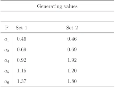
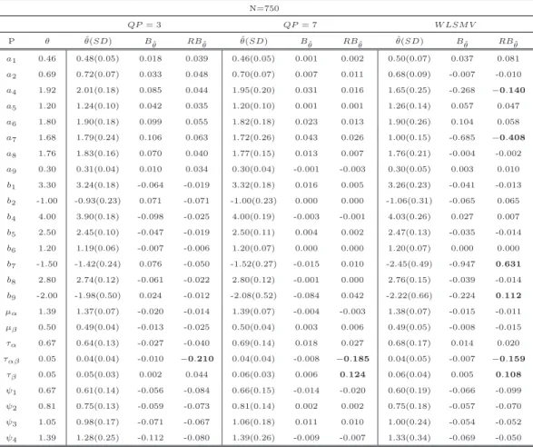
Table 2.1: Population Values for Item and Structural Parameters

Generating values

P Set 1 Set 2

a1 0.46 0.46

a2 0.69 0.69

a4 0.92 1.92

a5 1.15 1.20

a6 1.37 1.80

(38)

Table 2.1 – continued from previous page

Generating values

P Set 1 Set 2

a7 1.68 1.68

a8 1.76 1.76

a9 0.30 0.30

b1 2.30 3.30

b2 -0.50 -1.00

b4 3.00 4.00

b5 1.50 2.50

b6 1.00 1.20

b7 -0.30 -1.50

b8 2.00 2.80

b9 -1.00 -2.00

µα 1.39 1.39

µβ 0.50 0.50

τα 0.67 0.67

ταβ 0.05 0.05

τβ 0.05 0.05

ψ1 0.67 0.67

ψ2 0.81 0.81

ψ3 1.05 1.05

(39)

Table 2.1 presents the generating parameters employed in parameter set 1 and 2. Note

that for both parameter sets the only difference is the item parameters, with the structural

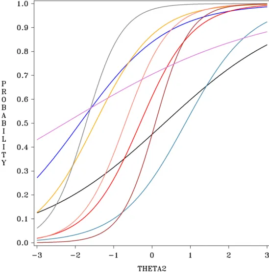
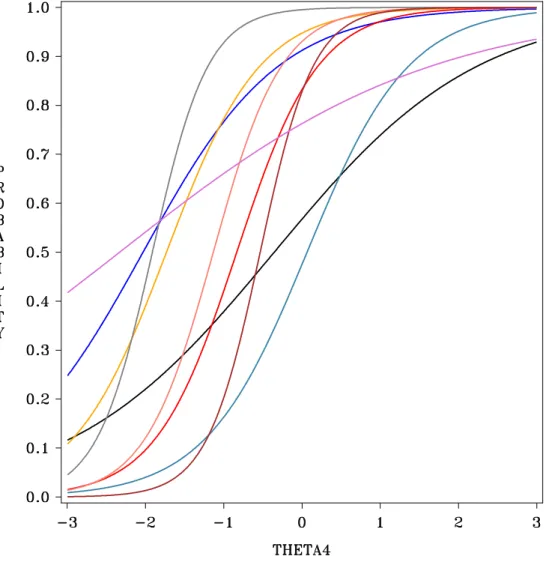
model parameters being fixed across sets. To characterize the difficulty range effect, ICC

plots for the two sets are plotted for each time-point. For ease of interpretation, the

ICCs are based on standardized parameters, and not the raw parameters listed in Table

2.1. The raw parameters were converted to the standardized metric using the following

procedure: Given

ϕkt=akt(θt₋bkt) _| θt _∼N(µt, σ_t2), (2.2)

I can obtain a standardized expression forϕkt under θt⋆ ∼N(0,1) by a Gaussian change

of variable function. Let

θ⋆t =

θt₋µt

σt → θ

⋆

t ∼N(0,1), (2.3)

then I can express

ϕ⋆_kt=a⋆_kt(θ_t⋆₋b⋆_kt)_| θ_t⋆ _∼N(0,1), (2.4)

where

a⋆_kt=akt_∗σt and b⋆_kt= bkt−µt

σt . (2.5)

As can be seen in the ICC plots for both sets, the generating procedure succeeded

in producing data which are representative of longitudinal studies of substance abuse or

internalizing behavior, in which the phenomenon of interest is rarely observed early on

and items are consequently difficult to endorse and not strongly discriminating, while

later in observation the phenomenon is more common and items appear less difficult

but more highly discriminating. Though both parameter sets were reflective of this

process, they differed in the range of θ measured by the scale. The first parameter set

was representative of a scale which measured a much more narrow range of the latent

construct, while the second parameter set measured a much broader range of the latent

(40)

expanding the range of the latent construct being measured resulted in a sparseness of

(41)

(42)

(43)

(44)

(45)

(46)

(47)

(48)

(49)

2.0.9 Implied Moments

The generating parameters given in Table 2.1 coupled with the coding of λ can be

used to calculate the implied moments of θ. As stated, the implied mean vector may

be calculated as µ_θ = λµ_η and the implied covariance matrix may be calculated as

Σθ=λτηλ

′ +ψ.

This resulted in

µ_θ=

1.392 1.892 2.392 2.892

(2.6)

and

Σθ =

        

1.34 ₋ ₋ ₋

0.7157575 1.6230301 ₋ ₋

0.761515 0.9072725 2.1060601 ₋

0.8072725 1.0030301 1.1987876 2.7890902          , (2.7)

with corresponding correlation matrix

Rθ=

        

1 ₋ ₋ ₋

0.4853446 1 ₋ ₋

0.4533052 0.490726 1 ₋

0.4175769 0.4714324 0.4946244 1

         . (2.8)

Because the structural parameters were held fixed across parameter sets, the implied

moments given here are the same for both parameter sets.

2.0.10 Sample Size Manipulation

All cells of the simulation were examined under two fixed sample sizes: N = 750 and

N = 3000. These sample sizes were chosen in order to minimize optimization problems

for WLSMV estimation under the wide difficulty range condition and because they were

representative of the large samples common in IRT applications. The lower sample size of

N = 750 was selected so as to be representative of what we considered to be a minimally

(50)

2.0.11 Non-Convergence

For every cell of the design, non-converged solutions were identified. Within a model

and parameter set combination, replications were fixed across estimator within sample

size cells. Thus, 300 replications were generated when N = 750 and each of these

replications was used in each estimator. Every unique replication which did not converge

across estimators was identified and within a sample size non-converged replications

were deleted and resampling of replications was conducted until a total of 300 converged

solutions were obtained in each sample size.

2.0.12 Improper Solutions

Following the work of Chen, Bollen, Paxton, Curran, and Kirby (2001) I

differ-entiated the importance of improper solutions (non-positive definite (NPD) covariance

matrices and negative variance estimates) based on the magnitude of the departure of

the parameter from its support. Thus, variance parameters for which estimates were only

slightly negative, or covariance matrices with eigenvalues that were trivially negative or

near zero were deemed to result from sampling variation, particularly when they were

associated with generating values which were themselves close to the boundary of

para-metric support. In addition, even when point estimates appear proper, the covariance

matrix may be degenerate, having a negative eigenvalue. Consequently, all variance

esti-mates were screened for degeneracy and replications having trivially degenerate solutions

were identified and described. These replications were not removed from analysis as this

could have induced a selection bias in the outcomes of interest. Rather, analyses were

conducted with results from all 300 converged replications. However, in order to assess

the potential impact of the degenerate solutions, sensitivity analyses, in which models for

bias were re-run omitting replications with improper solutions, were conducted to assess

(51)

CHAPTER 3

Results

To more clearly distill the experimental manipulation, and the fractional design

em-ployed, effects of interest related to sample size, estimator, model, and difficulty range

width are outlined in Table 3.1. This table also reflects the order with which results

are presented. First I will present results for Model 1 for the first and then second item

parameter sets, focussing on differences across sample size and estimator cells of the

design. This is then followed by the same presentation for Model 2. Convergence and

NPD solutions are discussed first. Bias and meta-model results are then discussed in

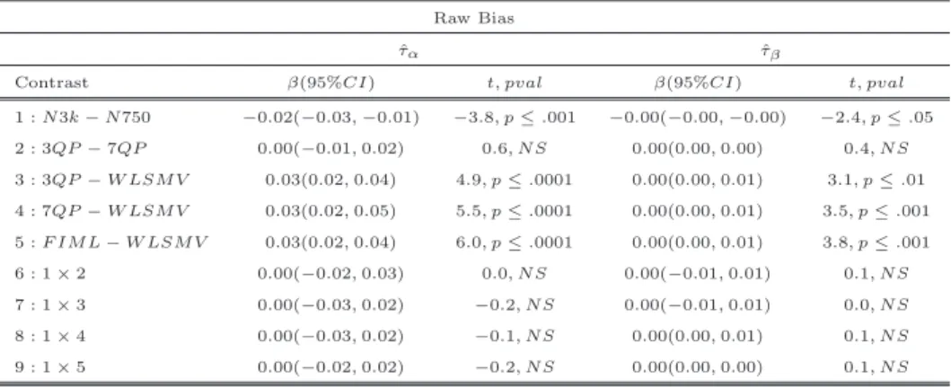
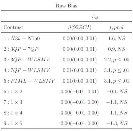
detail. Contrasts of interest in the meta-models include the sample size main effect, the

estimator main effects, and all sample size by estimator interactions. As detailed in the

results section, because patterns observed for RMSE did not differ from those for bias,

(52)

Table 3.1: Experimental Design

N = 750 & N = 3000

Estimator

Model Set Limited Information Full Information

1 1 W LSM V QP = 3 QP = 7

1 2 W LSM V QP = 3 QP = 7

2 1 W LSM V M CEM ₋

2 2 W LSM V M CEM ₋

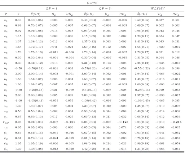
3.1 Model 1 3.1.1 Convergence

Non-converged replications were encountered only when estimation was based on

full information with three quadrature points per dimension. Of the 300 replications

simulated per cell, 40 failed to converge when N = 750, and 17 failed to converge when

N = 3000 under item parameter set 1. Under item parameter set 2, whenN = 750 a total

of 27 replications failed to converge, and when N = 3000 a total of 5 replications failed

to converge. The converged solutions corresponding to these replications were deleted

from the 7 quadrature point and WLSMV solutions. An additional 100 replications were

generated in order to replace the failed or deleted replications. This produced solutions

corresponding to 300 identical replications across all analyzed cells.

3.1.2 NPD Solutions

Under item parameter set 1, when N = 750 a total of 36 unique replications had

degenerate variance estimates. All estimates were associated with τη. A total of 8