aHuygens-Kamerlingh Onnes Laboratorium, Leiden Institute of Physics, Leiden University, Niels Bohrweg 2, P.O. Box 9504, RA Leiden NL-2300, the Netherlands bMathematical Institute, Leiden University, Niels Bohrweg 1, Leiden 23332CA, the Netherlands
cIBM T. J. Watson Research Center, 1101 Kitchawan Road, P.O. Box 218, Yorktown Heights, NY 10598, USA
A R T I C L E I N F O
Keywords:
LEEM
Low-energy electron microscopy Image registration
Detector correction Data analysis Parallel computation Spectroscopic imaging
A B S T R A C T
For many complex materials systems, low-energy electron microscopy (LEEM) offers detailed insights into morphology and crystallography by naturally combining real-space and reciprocal-space information. Its unique strength, however, is that all measurements can easily be performed energy-dependently. Consequently, one should treat LEEM measurements as multi-dimensional, spectroscopic datasets rather than as images to fully harvest this potential. Here we describe a measurement and data analysis approach to obtain such quantitative spectroscopic LEEM datasets with high lateral resolution. The employed detector correction and adjustment techniques enable measurement of true reflectivity values over four orders of magnitudes of intensity. Moreover, we show a drift correction algorithm, tailored for LEEM datasets with inverting contrast, that yields sub-pixel accuracy without special computational demands. Finally, we apply dimension reduction techniques to sum-marize the key spectroscopic features of datasets with hundreds of images into two single images that can easily be presented and interpreted intuitively. We use cluster analysis to automatically identify different materials within the field of view and to calculate average spectra per material. We demonstrate these methods by ana-lyzing bright-field and dark-field datasets of few-layer graphene grown on silicon carbide and provide a high-performance Python implementation.
1. Introduction
Low Energy Electron Microscope (LEEM) is a surface science tech-nique where images are formed from reflected electrons of low kinetic energy—down to single electronvolts. This is achieved by decelerating the electrons before they reach the sample and projecting them onto a pixelated detector after interaction with the sample. LEEM has proven to be a versatile tool, due to its damage-free, real-time imaging cap-abilities and its combination of electron diffraction with spectroscopic, and real-space information. This enables more advanced LEEM-based techniques such as dark-field imaging, where electrons from a single diffracted beam are used to create a real-space image, revealing spatial information on the atomic lattice of the sample[1,2].
Aside from usage as an imaging tool, LEEM is frequently used as a tool for quantitative analysis of physical properties of a wide range of materials. Multi-dimensional datasets can be created by recording LEEM images as a function of one or more parameters such as inter-action energyE0, angle of incidence, or temperature[3,4]. Using this, a
wide range of properties can be studied, for example, layer interaction, electron bands[5], layer stacking[2], catalysis[6], plasmons[7], and surface corrugation[8].
However, to unlock the true potential of quantitative analysis of multi-dimensional LEEM data, post-processing of images and combi-nation with meta-data is needed. In particular, it is necessary to correct for detector artifacts and image drift and to convert image intensity to physical quantities.
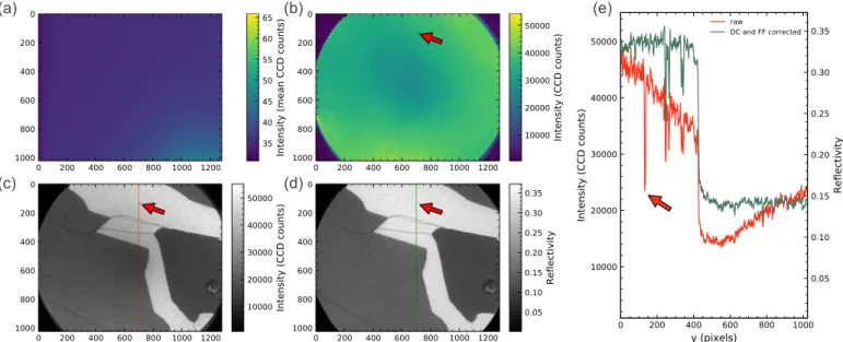
To this end, we here present a modular data acquisition and analysis pipeline for multi-dimensional LEEM data, combining techniques well established in other fields such as general astronomy or transmission electron microscopy (TEM), that yields high resolution spectroscopic datasets and visualizations thereof. In particular, starting with the raw data (shown inFig. 1(a)), we correct for detector artifacts using flat field and dark current correction. Combining these corrections on the images with active feedback on detector gain enables High Dynamic Range (HDR) spectroscopy, which makes it possible to measure spectra over four orders of magnitude of intensity. Subsequently, we
https://doi.org/10.1016/j.ultramic.2019.112913
Received 12 July 2019; Received in revised form 13 November 2019; Accepted 22 November 2019 ⁎Corresponding author.
E-mail address:[email protected](T.A. de Jong).
Available online 23 November 2019
demonstrate that compensation of detector artifacts also enables drift correction with sub-pixel accurate image registration, yielding a fully corrected data stack (Fig. 1(b)). This creates a true pixel-by-pixel spectroscopic dataset, as shown inFig. 1(c), i.e. every pixel contains a reflectivity spectrum of the corresponding position on the sample. Fi-nally, we explore the potential for more advanced computational data analysis. We show that by using relatively simple dimension reduction techniques and clustering, these datasets can be intuitively analyzed and visualized, enabling semi-automatic identification of areas with different spectra.
To demonstrate these features and quantify the accuracy, we apply the drift correction algorithm to artificial data and then apply the full pipeline to a real dataset acquired on the SPECS P90 based ESCHER system in Leiden[9–11]. The sample of the dataset is few-layer gra-phene grown by thermal decomposition of Silicon Carbide (SiC)[12], followed by hydrogen intercalation to decouple the graphene from the SiC substrate [13,14]. Bright Field LEEM spectra can be used to dis-tinguish the resulting mixture of bilayer, trilayer and thicker graphene, as interlayer states cause distinct minima in the reflectivity spectra[15,16]. In addition, the growth process causes strain-induced stacking domains, which can be distinguished using Dark Field LEEM spectra[2,17]. The sample dataset consists of bright-field and dark-field LEEM images of the same area for a range of landing energies (some-times referred to as LEEM-I(V)). The dark-field dataset uses a first order diffraction spot and tilted illumination such that the incident beam has the opposite angle to the normal as the diffracted beam, as described in more detail in Ref. [2]. The data is available as open data[18]and is interpreted and investigated in detail in Ref.[2,19].
2. Detector correction
No physical detector system is perfect, i.e. each detector system introduces systematic errors and noise. Knowledge of the sources of these imperfections enables the correction of most of them. The ESCHER LEEM has the classical detector layout: A chevron micro-channel plate array (MCP, manufactured by Hamamatsu) for electron multiplication, a phosphor screen to convert electrons to photons and a CCD camera (a PCO sensicam SVGA) to record images of the phosphor screen.
The CCD introduces artifacts in the form of added dark counts and a non-uniform gain[20–23]. Furthermore, the MCP gain is also spatially non-uniform, for example due to overexposure damaging of the MCP, resulting in locally reduced gain. Therefore we describe the measured intensity ICCD on the CCD as the following combination of the
previously named detector artifacts and the ‘true’ signalIin:
= +
ICCD( , )x y DC x y( , ) I x y G x yin( , )· ( , ) (1) whereDC(x, y) is the intensity caused by dark current andG(x, y) is the position-dependent and as-of-yet unknown gain factor comprisingall modifications to the gain due to the complete detector system com-prised of the MCP, phosphor screen and CCD camera together.
To compensate for these detector artifacts, we employ techniques well-established in astronomy (and other fields using CCD cameras) to effectively invert the relation inEq. (1), to extractI x yin( , )without the deleterious effects of background dark countsDC(x, y) and local gain variationsG(x, y).
First, the dark current of the CCD is compensated by pixel-wise subtracting a non-illuminateddark countimage, i.e. an image with the same exposure time as used for the measurement, but no electron il-lumination at all. A pixel-wise average of a set of such dark count images is shown in Fig. 2(a). The dark current arises from thermal excitations in the sensor and varies over time with an approximately Gaussian distribution. The mean of this distribution is dependent on the pixel, i.e. thex, ylocation, for example visible inFig 2(a) as a slight increase in the lower right corner. To suppress the thermal fluctuations in the template dark current image, it is desirable to average over several dark count images to prevent the introduction of systematic errors. We assume that the per-pixel dark currents are identically dis-tributed with a varianceVarthermexcept for a spatial varianceVarspatialof the mean. This is mathematically equivalent to assuming the dark current fluctuates around its mean with both spatially dependent (but fixed in time) noise and time-dependent thermal noise. By averaging multiple dark images, we reduce the thermal variance but not the spatial variance. The remaining variance is given by:
= +
= +
n n
n
Var ( ) Var ( ) Var
1
Var (1) Var
tot therm spatial
therm spatial
Where Var(n) is used to denote the variance ofnpixel-wise averaged images. By determiningVar ( )totn andVar (1)tot experimentally we can isolate the thermal noise on a single image:
= n n
n
Var (1) Var (1) Var ( ) ·
1
therm tot tot
(2) For the ESCHER system with its Peltier-cooled camera, we find
× =
Vartherm(16 250ms images) 114.3. Therefore, a set of 120 × 16
images (a total exposure time of 8 minutes) is sufficient to suppress the systematic errors to values smaller than the discretization error. We
find that the dark count image does not significantly change over time, and therefore remeasuring dark count images is seldomly needed.
Second, to compensate for spatial gain variations, which are mostly due to the MCP, a (conventional)flat fieldcorrection is performed, di-viding the full dark count-corrected dataset by an evenly illuminated image[24]. In LEEM, when the potential of the sample corresponds to a higher potential electron energy than the kinetic energy of the electrons of the beam, all incoming electrons turn around before they reach the sample. In this situation the electron landing energy is negative and the sample behaves as a mirror. Imaging at a landing energy ofE0 20eV yields an almost perfect flat field image as approximation ofG(x, y) in Eq. (1). A relatively large value for the negative energy is taken to prevent artifacts from local in-plane electric field components, e.g. due to work function or height differences in the sample[25–27]. For the ESCHER system, it is necessary to take flat field images within hours of the measurement, as the MCP wears over time and the gun emission profile and system alignment change on relatively short time-scales[28]. Furthermore, taking a flat field image at the same precise alignment as the measurement is preferred for two reasons. First, bar-ring absolutely perfect alignment of the system as well as a perfectly uniform emission from the electron gun, the beam intensity is not spatially uniform. As illumination inhomogeneities are dependent on the precise settings of the lenses, these will also be compensated for if the flat field is recorded in the exact same configuration. Second, for proper normalization of the data, as explained inSection 3, the same magnification (projector settings) is needed.
An alternative to this mirror mode flat fielding is to average over a sufficiently large set of images of different positions on the sample and use the resulting average as a flat field image. In most cases however, mirror mode flat fielding is preferred over such ensemble-average flat fielding since for the latter many images of different locations are re-quired. Even when such a set is already available, it is hard to rule out any systematic (statistical) errors. Lastly ensemble-average cannot provide proper normalization of the data to convert to true reflectivity.
3. High dynamic range spectroscopy
In LEEM and LEED, large variations occur in the amplitude of the signal, both within individual images and from image to image. For
example, in quantitative LEED, features of interest are often orders of magnitude less bright than primary Bragg peaks. This necessitates a detector system with a large dynamic range. The CCD-camera of the ESCHER setup has a bit depth of 12 bits and a possibility to accumulate 16 images in hardware, yielding an effective bit depth of 16 bits for singular images.
For most materials, the reflected intensityI(E0) changes over orders of magnitude as a function ofE0. Starting in mirror mode with unity reflectivity, the reflected intensity tends to decrease orders of magni-tude forE0≲100eV. To obtain spectra with such a large dynamic range, the dynamic range offered by the bit depth of the CCD alone is not sufficient.
However, the gainGof the MCP, i.e. the ratio of outgoing electrons to incoming electrons, can be tuned by the voltageVMCPapplied over
the MCP. This gain scales approximately exponential inVMCP (over a
reasonable range, see next section), enabling image formation of ap-proximately constant intensity on the CCD, for a wide range of incident electron intensities. We use this property to develop a scheme to further increase the dynamic range in whichG V( MCP)is adjusted by setting a
new MCP bias for each new image, i.e. increasing the gain for images where the reflected intensity is low. MeasuringVMCPfor each recorded
image and calibratingG V( MCP) makes it possible to employ the full
dynamic range of the CCD-camera for all landing energies, without losing the information of the absolute magnitude of the measured in-tensities, thus extending the range of spectroscopy without significant decrease in signal-to-noise ratio.
3.1. Calibration
Hamamatsu Photonics K.K., the manufacturer of the microchannel plate in the ESCHER setup, specifies an exponential gain as function of voltage for a part of the range of possible biases[29]. To extend the useful range beyond this limit and thus enable the use of the full bias range up to the maximal 1800 V, the gain versus bias curve was cali-brated as follows:
1. First, in mirror mode,VMCPis adjusted such that the maximum
in-tensity in the image corresponds to the full inin-tensity on the CCD, staying just below intensities damaging the MCP.
2. While decreasingVMCP,images are acquired for evenly spaced bias
values. The intensities of these images form the dataset for cali-bration of the low bias part.
3. ReturningVMCPto the previous maximum value,E0is increased until the intensity of the image is so low that it is barely distinguishable from the dark count.
4. AgainVMCPis turned up until the maximum image intensity
corre-sponds to the maximum CCD intensity.
5. Steps 2. to 4. are repeated until a dataset is acquired starting at maximum MCP biasVMCP. The resulting average intensity curves are
shown inFig. 3(a).
6. These datasets are then corrected for dark count as discussed above, resulting in the average intensity curves shown inFig. 3(b). Com-paring to the uncorrected curves, the increase in accuracy for low intensity values, crucial for accurate calibration, is very apparent. Averaging over a sufficiently large area ensures sufficient reduction of other noise sources such as MCP noise.
7. A joint fit ofEq. (3), allowing for a different amplitudeAifor each curve, is performed to the corrected data to obtain a general ex-pression for MCP gainGas a function ofVMCP. The fit is performed
using least squares on the logarithm of the original data with no additional weights, to ensure a good fit over the large range of or-ders of magnitude. The fitted curve is then normalized to a con-venient value, e.g. G(1 kV)=1. This normalization can be freely chosen, asGwill be applied equally to datasets and flat field images, yielding absolute reflectivity as resulting data.
A first choice for a fitting function would be a simple exponential, but this would not account for any deviation from perfect exponential gain, visible as deviations from a straight line inFig. 3(b). For the ES-CHER setup we therefore choose to add correction terms of odd power in the exponent:
=
=
+ G V( ) Aiexp c V
k
k k
MCP
0 8
MCP2 1
(3) Only odd powers were used to accurately capture the visible trends in the data. For the ESCHER setup correction terms up to orderVMCP17
(k< 9) turned out to give a satisfactory good approximation, as illu-strated by the residuals inFig. 3(d).
3.2. Active per-image optimization of MCP bias
The resulting curve with calibration coefficients is then used to actively tune the MCP bias during spectroscopic measurements: A de-sired range is defined for the maximum intensity on the camera, cor-responding to a maximum safe electron intensity on the MCP to prevent damage on the one hand, and a minimum desired intensity of the image on the CCD on the other hand. Whenever the maximum intensity of an
image falls outside this range, the MCP gainG(V) will be adjusted such that the intensity of the next image again falls in the center of this range. Assuming the intensity changes continuously, this method en-sures the use of the full intensity range of the camera for each image, while protecting the MCP against damage.
Additionally, after the measurements, the calibration curve is used to calculate the real, relative intensity from the image intensity and the recordedVMCP. By dividing this intensity by the intensity of the flat field
image (taken in mirror mode and corrected for dark current and the MCP bias), we calculate a (floating point) conversion factor to true reflectivityvalues for each image. These ratios are added to the metadata of every image. By applying this conversion as a final step after any analysis of the data, errors due to discretization of highly amplified, and therefore low true intensity, images are minimized. Note that this procedure makes the conversion to true reflectivity possible even for datasets with no mirror mode in the dataset itself, such as dark field measurements.
3.3. Comparison of results
Spectroscopic LEEM-I(V) curves on bilayer graphene on silicon carbide are measured both with constant MCP bias and with adaptive MCP bias as described above. A comparison between the resulting curves is shown inFig. 4. While the regular, constant MCP, curve starts to lose detail aroundE0=50eV,i.e. after a factor of 100 decrease in
signal, the adaptive measurement captures intensity variations in the spectrum almost 4 orders of magnitude lower than the initial intensity. We thus call the adaptive method high dynamic range (HDR) imaging.
4. Drift correction by image registration
In LEEM imaging, the position of the image on the detector tends to shift during measurement as shown inFig. 1(a). This prevents per-lo-cation interpretation of the data, both for spectroscopic measurements and measurements with varying temperature. Although the shift can be minimized by precise alignment of the system, we find that a significant shift always remains, especially in tilted illumination experiments such as DF-LEEM or angle-resolved reflected-electron spectroscopy (ARRES)[2,4,27], which makes the compensation of this image drift necessary.
This problem has been studied in depth in the field of image re-gistration, motivated by wide-ranging applications such as stabilization of conventional video, combination of satellite imagery and medical imaging[30–32]. Techniques generally rely on defining a measure of similarity between a template and other images, either by some form of cross correlation, or by identifying specific matching features in both. The image is then deformed by a fixed set of transformations (either affine, i.e. purely shifts and rotations or non-rigid, i.e. additional
deformation), until the match between the features in the images and the features in the template is maximal. For LEEM data, the measure-ment drift is almost completely described by in-plane shifts, sig-nificantly reducing the space of expected transformations. A common approach in this case is to use the (two-dimensional) cross-correlation as a measure of similarity between two shifted images and to find the maximum for all images compared to a template, as the location of maximum of the cross-correlation corresponds directly to the shift be-tween the image and the used template.
The cross correlation of twon×npixels imagesI1(x, y) andI2(x, y) is defined as follows:
= + +
= =
I I x y
n I x y I x x y y
( , )( , ) 1 ( , ) ( , )
x n
y n
1 2 2
0 1
0 1
1 2
(4) where the coordinates can be wrapped around, i.e. all spatial co-ordinates are modulon. Furthermore, we can relate this to the con-volution operation (denoted as∘):
= =
= =
I I x y I x y I x x y y
I x y I x y x y
( , )( , ) ( , ) ( ( ), ( ))
: ( ( , ) ( , ))( , ) n nx ny
1 2 1 10 10 1 2
1 2
2
(5) Using this, the cross correlation can be expressed in terms of (two-di-mensional) Fourier transforms :
= =
I I I x y I x y I I
( , )1 2 1( , ) 2( , ) 1( ( )· ( ))1 2 (6)
Where ( )I2 denotes the complex conjugate of the Fourier transform of
image 2. This makes the cross-correlation extra suitable as a measure of similarity, since it can be computed efficiently using the two-dimen-sional Fast Fourier Transform (FFT). Determining the local maximum of the cross-correlation yields the integer shift for which the two input images are most similar, with the height of the maximum an indication of the quality of the match. To further increase accuracy, several var-iants, such as gradient cross-correlation and phase-shift cross-correla-tion, have been shown to achieve sub-pixel accuracy for pairs of images[30,33–35].
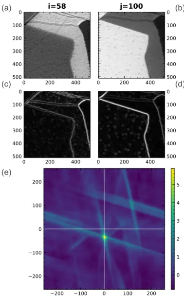
For LEEM data however, the straightforward cross-correlation ap-proach is often hindered by the physics underlying the electron spectra, resulting in contrast changes (c.f.Fig. 5(a,b)) and even inversions for different values ofE0. The problem can be slightly alleviated by using multiple templates, but in general this approach is unsatisfactory. In-stead we present another approach here: We first apply digital filters
and then compare each image to all other images, similar to the algo-rithm by Schaffer et al. for energy filtered transmission electron mi-croscopy[36]. It then uses a statistical average of the found integer shifts between all pairs of images to achieve sub-pixel accuracy.
We analyze the accuracy of this algorithm using an artificial test dataset and show that the accompanying Python implementation[37] is fast enough to process stacks of hundreds of images in mere minutes by performing benchmarks on a real dataset, followed by a discussion of the algorithm and results.
The algorithm consists of the following steps:
1. Select an area of each of the (detector-corrected)Nimages, suitably sized for FFTs (i.e. preferably 2n× 2npixels).
2. Apply Gaussian smoothing with standard deviation ofσpixels to reduce Poissonian noise in the images.
3. Apply a (magnitude) Sobel filter to highlight edges only, as shown in Fig. 5(c) and (d). As such, images with inverted contrast (c.f. Fig. 5(a) and (b)) become similar to each other.
4. UsingEq. (6), compute the cross-correlation, as shown inFig. 5(e). Do this for all pairs (i, j) of images.
Fig. 4.Regular spectroscopic reflectivity curve (orange) of bilayer graphene on SiC, corrected for dark count and flat field, but with a single setting ofVMCP(top panel). The HDR measurement of the same area with active MCP bias tuning (blue) can resolve details down to lower intensity. (For interpretation of the references to colour in this figure legend, the reader is referred to the web version of this article.)
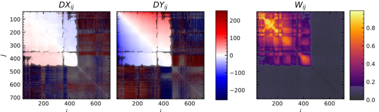
5. Compute the location (DX, DY)ijand valueWijof the maximum of the cross-correlation for all image pairs (i, j).DXijandDYijform the anti-symmetric matrices of found relative shifts in either direction, whileWijis a symmetric matrix of weights of the found matches, as shown inFig. 6.
6. Normalize the maximum valuesWijto be used as weights in step 8:
=
Wij W WWii·ij jj.
7. Pick a thresholdWminto remove any false positive matches between images. A threshold ofWmin =0.15, based onDX, DY andWij, is shown inFig. 6as gray shading. SetWij=0for allWij<Wmin. 8. To reduce theN2relative shiftsDXto a lengthNvector of horizontal
shifts dx, minimize the errors (dxi dxj DX Wij) ij4 (using least squares). Do the same withDYto obtain the vertical shift vectordy. 9. Apply these found shiftsdxanddyto the original detector corrected images, interpolating (either bi-linearly or via Fourier) for non-in-teger shifts.
4.1. Accuracy testing
To validate and benchmark the accuracy of the drift correction al-gorithm beyond visual inspection of resulting drift corrected datasets, an artificial test dataset with known shifts was created. This enables exact comparison of results to a ‘true’ drift.
The test dataset, as shown inFig. 7, consists ofN=100copies of an annulus of intensity 1.0 on a background of 0.0. The dataset is shifted over a parabolic shift in thex-direction and random shifts uniformly chosen from the interval [ 0.5, 0.5] pixels in the y direction (see Fig. 7(a)). Finally pixel-wise Gaussian (pseudo-) random noise is added to all images. The standard deviationAof the added random noise is then varied to simulate images with different signal-to-noise ratios (SNR).
The resulting maximum error in the found shift compared to the original, ‘true’ shift, as well as the resulting mean error for different values ofAandσis shown inFig. 8, separately for thexandy direc-tions. These results verify that, at least for synthetic datasets, the al-gorithm achieves sub-pixel accuracy, with the mean absolute error in pixels of about 0.1 times the relative noise amplitudeAfor the optimal value of smoothingσ, and the maximum absolute error just reaching 0.5 pixel for the extreme value of A=2. As expected, the error is strictly increasing for decreasing SNR, i.e. increasingA. After an initial cutoff, visible in saturated yellow inFig. 8, the accuracy of the algo-rithm is also generally decreasing for increasing smoothing widthσ. However, after this initial cutoff, there is a comfortably large range ofσ where the algorithm performs well.
The choice of smoothing parameter σ has significant influence on the analysis of real data, as is visible inFig. 6: for highE0, the noise level is so high that no feasible matches were found for the used value of smoothing σ. Increasing σ alleviates this, but reduces the match quality for images with low noise level.
We found that most features visible in the high-σ, high-Aregime of Fig. 8(b,d) are dependent on the initialization of the random generator for the added pixel-wise noise and are thus not significant (c.f. a second run in Supplementary Fig. A.1).
4.2. Time complexity
To benchmark the computational complexity of the algorithm, it was applied to subsequently larger parts of the real dataset, while measuring the computation times for the least squares optimization (step 8 above) and the shifting and writing of images (step 9) sepa-rately. The results show calculating the cross-correlations takes the most time, as it scales almost perfectly quadratically in the number of
Fig. 6.Calculated shift matricesDXandDYand weight matrixWijfor the bright-field dataset. Matches of a weight belowWmin=0.15(shaded in gray) are mostly false positives. Consequently, they are set to zero weight in the algorithm.
imagesN, as shown inFig. 9. The shifting and writing of images scales linearly and is not significant for larger datasets. The total time there-fore scales nearly perfectly quadratically, with a dataset of 500 images drift corrected in less than 7 minutes of computation time (exact details of the hardware and software used for benchmarking can be found in the Supplemental Information). As such, LEEM spectroscopy datasets can be comfortably and regularly drift corrected on a desktop PC. 4.3. Discussion
We elaborate here on the choices made in the algorithm. The use of the magnitude Sobel filter has multiple benefits, similar to using the gradient cross-correlation: Contrast inversions between areas with dif-ferent spectroscopic properties nonetheless result in similar images (c.f. Fig. 5(c,d)). In addition, the constant zero background reduces errors due to wrap-around effects due to performing the calculation in the
Fourier domain.
The exponent 4 for the weighing matrix Wijin the least squares minimization step 8 was empirically found to give the best results for real datasets.
As already noted by Schaffer et al., the use of cross-correlation be-tween multiple image pairs and combining the returned integer shift values enables sub-pixel accuracy. The maximum theoretical accuracy isN1 pixels,but is reduced for images where false positive matches are thresholded out.
Alternative methods of obtaining sub-pixel accuracy in determining shifts include a combination of upscaling and matrix-multiplication discrete cosine transforms[34]and a rather elegant interpolation of the phase cross-correlation method proposed by Foroosh et al.[30]. How-ever our current method is less complex and combines robustness against global drift with handling of changing contrasts, which is cru-cial for spectroscopic LEEM data. Although the sub-pixel precise phase
Fig. 8. (a,b)Maximum and mean error indxshift as calculated by the algorithm for different values of noise amplitudeAand smoothing parameterσ. The optimal value of the Gaussian smoothingσas a function of added noise amplitudeAis drawn in white. Black contour lines are added as a guide to the eye.(c)Spread of the error for the optimal values ofσfor varyingA. Dark and light bands are respectively 1 and 2 standard deviations, maximum error is indicated as gray line.(d,e,f) Same for theydirection.
correlation method seems a straightforward extension of regular cross correlation, it is less suitable for datasets with changing noise levels and not suitable for false positive detection by normalization, both prop-erties we found essential to handle spectroscopic LEEM data.
Fourier interpolation for non-integer shifts, corresponding to Whittaker–Shannon interpolation, is optimal when the image resolution is limited by the optical transfer function of the intstrument, instead of pixel sampling-limited[38]. In this case, almost always true for LEEM measurements, the imaginary part is zero up to floating point precision and can be discarded. If however the resolution is limited by the de-tector, e.g. at very low magnifications, bi-linear interpolation is the better choice.
Contrary to Schaffer et al., we found smaller values of Gaussian smoothing width σyield the best results, with larger values yielding artificial shifts around contrast inversions for real datasets and gen-erally performing worse for the synthetic dataset, as visible inFig. 8.
Schaffer et al. found their approach at the time (2004) not com-putationally feasible for large amounts of images but, as shown in the previous section, the current implementation is able to drift correct a stack of several hundreds of images comfortably on a single desktop computer. We want to emphasize that the use ofPythongives flex-ibility and makes it easy to adapt the code. For instance, increasing performance even more lies within reach by performing the FFT cross-correlations and maximum search on one or more graphical processing units using one of several libraries or by using a cluster running adask scheduler. Further speedup would be possible by pruning which pairs of images are to be cross-correlated. An avenue not explored here, is the use of pyramid methods to create a multi-step routine where firstly a fast estimate of the shift is computed on a smoothened and reduced-size image before using consecutively larger images to refine the esti-mate[39,40].
Beyond drift correction, the same method presented here can also be applied to create precisely stitched overview images of areas much larger than the electron beam spot size. Although, as no contrast in-versions or large feature differences are expected for the matching areas, the added value of using a gradient filter is nullified. Additionally the number of images that can be matched to the same template is limited, forcing a low upper bound on the sub-pixel accuracy of the optimization part of the algorithm. Instead, we found that an algorithm based on more regular phase-shift cross-correlation is sufficient for sub-pixel accurate stitching.
5. Dimension reduction
The sub-pixel accuracy drift correction now makes it possible to reinterpret a LEEM-I(V) dataset as a truly per-pixel set of spectroscopic curves, opening up possibilities for further data analysis. For a dataset
ofNimages, each such curve (c.f.Fig. 1) can be seen as a vector in aN -dimensional vector space of the mathematically possible spectra. Even for moderate datasets of a few hundred images this is a huge vector space. In almost all cases however, the physical behavior of the data can be described with a model with far fewer degrees of freedom, i.e. the vector space of physically possible spectra has a much lower number of dimensions. Therefore, it should be possible to summarize all sig-nificant behavior in a much smaller dataset, which can be analyzed (and visualized) much more easily.
Here, we use Principal Component Analysis (PCA), a linear tech-nique based on singular value decomposition (SVD), often used for dimension reduction in data science fields[41–43]. The randomized iterative variant of PCA allows for efficient computation of the largest variance components without performing the full SVD decomposi-tion[44]. This technique therefore projects the spectroscopic data to a lower dimensional subspace, in such a way that maximal data variance is retained. It does so in a computationally efficient way, making it well suited for, and popular in, data science. Before applying PCA, we crop the dataset to remove any areas that lie outside of the detector for any image inside the used range ofE0. Additionally, each image is scaled to zero mean and unit variance, to not let brighter images contribute more strongly to the analysis as they have larger variance. A lot of other choices for standardization of the data are possible, most of them with useful results, but for the scope of this paper we adhere to this standard choice.
After performing PCA, the lower dimensional subspace or PCA-space, is now spanned by orthogonal ‘eigen-spectra’, referred to as PCA components. Since the projection map onto this subspace retains most of the variance in the dataset, it is possible to build an approximate reconstruction of the full physical spectra from the reduced PCA spectra.
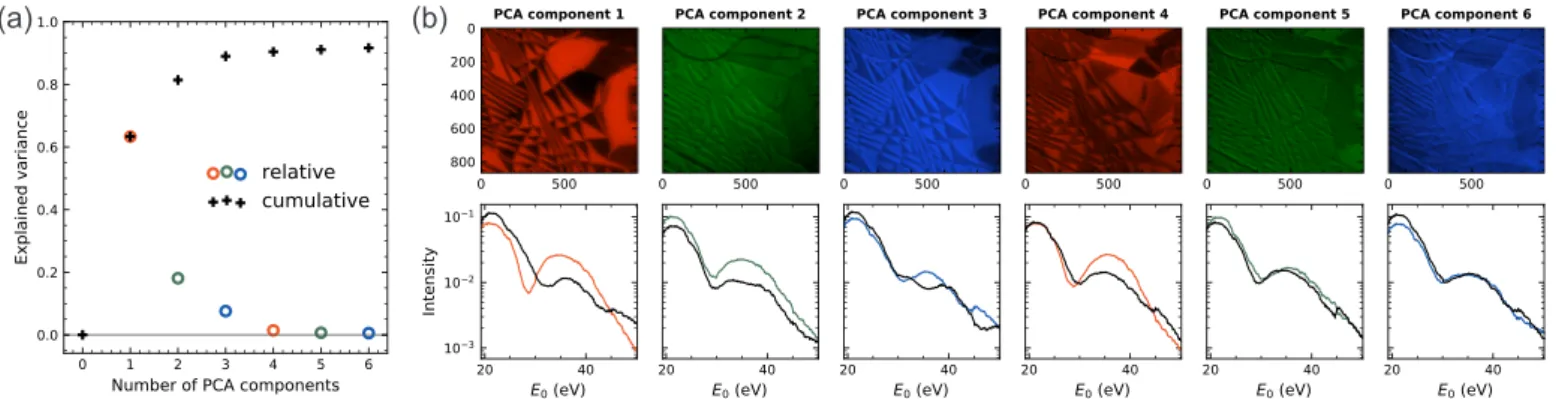
Although the aim is dimension reduction, the number of PCA di-mensions should be chosen large enough, such that the mathematical PCA-space contains all physical behaviour up to a certain noise level[45]. A so-called scree plot, displaying the captured variance, aids to pick the right number of dimensions. For the sample dataset of dark-field images ofN=300energies, a scree plot is shown inFig. 10(a). In general, for spectroscopic LEEM datasets, we find that reducing down to 6 dimensions is often enough to capture more than 90% of all variance. The dataset can be projected onto a single PCA component by taking the per-pixel inner product with the corresponding ‘eigen-spectrum’. This yields images visualizing the variance retained by the respective components, as shown in the top half ofFig. 10(b) for all 6 PCA com-ponents. Below each image, the spectra corresponding to the pixels with the minimum and maximum value of this projection are shown in black and color, respectively.
5.1. Visualization
Reducing a spectrum from hundreds of dimensions to a few opens up new opportunities for data visualization. In particular, it allows for the visualization of nearly all of the variation in spectra of an entire dataset in only two images, as shown inFig. 11. Here, the values of the six principal components (c.f.Fig. 10), are displayed as the RGB color channels of two pictures per dataset. To lift the degeneracy in the possibilities of the sign of the PCA components (a PCA eigen-spectrum with the opposite signs retains as much variance), we change the signs such that the a positive projection onto the PCA component corresponds to having the higher average relative brightness in the images. This way, areas that are bright in the majority of the original images also appear bright in the visualization. To compensate for the human eyes’ preference for green, a scaling of colors as proposed by Kovesi is ap-plied[46]. It is given by the following matrix:
=
R G B
R G B 0.90 0.17 0.00 0.00 0.50 0.00 0.10 0.33 1.00
The results are striking. All the sample features are directly visible inFig. 11: In the bright field dataset, bilayer and thicker graphene are clearly separated in orange and green, respectively in the first three PCA components [Fig. 11(a)]. Moreover, SiC step edges, domain walls and point-like defects are clearly visible. The next three PCA
components [Fig. 11(b)] highlight the difference between bilayer (green), trilayer (orange) and four-layer graphene (dark green) and in addition separates step edges (orange), domain boundaries (turquoise) and the defects in different colors. Furthermore, two types of domain boundaries can be observed in the four-layer area that are hard to tell apart in conventional LEEM images. The light green and dark ones are presumably domain boundaries in the top-most and lower layers, re-spectively.
This visualization using the first three PCA components of the dark field dataset [Fig. 11(c)] clearly separates the different stacking orders in bilayer (AB in orange and AC in blue) and trilayer graphene. The PCA components 4 to 6 [Fig. 11(d)] highlights the different stacking orders in trilayer and four-layer areas (different shades of orange and blue) and display an interference effect causing double lines at one type of (corresponding to one direction of) domain edge. This clear visualiza-tion is particularly remarkable as the dark-field dataset presents a worst case scenario due to its extreme off-axis alignment (see [2]for full details), which causes strong image drift and relative shifts of features. 5.2. Clustering and automatic classification
In addition to the visualization possibilities explored in the previous section, the dimension reduction by PCA lowers the complexity of the data enough to enable the use of other, more quantitative data analysis techniques. In particular, reduction to less than ten dimensions is
enough to perform unsupervised classification or clustering on the en-tire dataset. Here, we show that a relatively simple clustering algo-rithm, the classical k-means, also known as Lloyd’s algorithm [47], applied to the PCA reduced dataset, can already be used to distinguish the relevant, different areas. The structure of the bright field dataset is visualized in terms of the first three PCA components inFig. 12(a), both as a point cloud with colors corresponding toFig. 11(a) and as density projections (gray scale) on the three planes. The resulting classification from the application ofk-means to the six PCA components is visualized in the same way inFig. 12(b), where the color of the points now cor-responds to the assigned labels. These same label colors are shown in real space inFig. 12(c). In the real space visualization it is clear that the different layer counts are separated (bilayer, trilayer and four-layer as purple, orange and red, respectively) from a class with the point defects and step edges (blue) and a class containing the domain boundaries in the bilayer (green). The cluster labels can now be used to calculate spectra of each area, e.g. all trilayer pixels without the defects. For this, we take the mean over all pixels belonging to one cluster for each ergy in the full N-dimensional dataset. This can be done even for en-ergies outside the range used for the initial clustering as well as for energies where we only have partial data due to drift. The resulting spectra for the clustering inFig. 12(c) are plotted inFig. 12(d).
The same clustering method is applied only to the first 4 PCA components of the dark-field dataset since component 5 and 6 show virtually no distinguishing features and corresponds to very little var-iance [cf.Fig. 10(a,b)]. The resulting real space labeling of the clusters and the spectra are shown inFig. 12(e) and (f), respectively. Here, al-though not perfect, the clustering algorithm manages to mostly separate the different possible stacking orders (red and orange for the bilayer and purple, brown, pink and blue for the trilayer). The green and gray areas correspond to areas where clear classification as a stacking order
is not possible due to phase contrast and non-uniform illumination ar-tifacts due to the tilted illumination.
Thanks to the proper calibration and mutual registration of the data, this relatively simple algorithm classifies the areas in the dark-field data set with only minor errors (e.g. the incorrect assignment of brown tri-layer spectrum in the lower left),withoutany input of the positions of each spectrum in the image or any input about the expected differences between spectra. We anticipate that this classification using un-supervised machine learning will be useful for identifying unknown spectra in new datasets.
6. Conclusion
We have shown that treating (energy-dependent) LEEM measure-ments as multi-dimensional datasets rather than as collection of images, opens rich opportunities for detailed and quantitative insights into complex material systems that go well beyond morphological and crystallographic characterization.
Three key steps are necessary to convert a stack of raw LEEM images into spectroscopic dataset with a greatly increased body of quantitative information. First, we compensate for common detector artifacts such as camera dark count and non-uniform detector gain, which is crucial to quantitatively interpret LEEM images. Second, by calibrating the channel plate gain and adjusting it during spectroscopic measurements, we can not only extend the dynamic range of the dataset by two orders of magnitude, but also convert image intensity into absolute reflectivity or electron intensity (provided the beam current is accurately mea-sured). Third, we describe a drift-correction algorithm that is tailored for spectroscopic LEEM datasets where contrast inversions make many other approaches unfeasible. It relies on digital filtering and cross-correlation of every image to all other images and, without requiring
Treating LEEM measurements as multidimensional datasets as pre-sented here will further strengthen the role of LEEM as a quantitative spectroscopic tool rather than as a pure imaging instrument, thus deepening its impact in the research and discovery of novel material systems. Furthermore, the presented techniques can be applied to re-lated spectroscopic imaging techniques, such as energy-filtered PEEM[49]or even adapted for use in scanning probe techniques such as scanning tunneling spectroscopy[42,50]. To facilitate the use of the approaches discussed here, the test data as well as Python code is available online[18,37].
Declaration of Competing Interest
The authors declare that they have no known competing financial interests or personal relationships that could have appeared to influ-ence the work reported in this paper.
Acknowledgements
We thank Marcel Hesselberth and Douwe Scholma for their indis-pensable technical support and Christian Ott and Heiko Weber for the fabrication of the graphene on SiC samples. Funding: This work was supported by the Netherlands Organisation for Scientific Research (NWO/OCW) via the VENI Grant No. 680-47-447 (J.J.); and as part of the Frontiers of Nanoscience program.
Supplementary materials
Supplementary material associated with this article can be found, in the online version, atdoi:10.1016/j.ultramic.2019.112913.
References
[1] E. Bauer, M. Mundschau, W. Swiech, W. Telieps, Surface studies by low-energy electron microscopy (LEEM) and conventional UV photoemission electron micro-scopy (PEEM), Ultramicromicro-scopy 31 (1) (1989) 49–57,https://doi.org/10.1016/
0304-3991(89)90033-8.
[2] T.A. de Jong, E.E. Krasovskii, C. Ott, R.M. Tromp, S.J. van der Molen, J. Jobst, Intrinsic stacking domains in graphene on silicon carbide: a pathway for inter-calation, Phys. Rev. Mater. 2 (10) (2018) 104005,https://doi.org/10.1103/ PhysRevMaterials.2.104005.
[3] J.I. Flege, E.E. Krasovskii, Intensity-voltage low-energy electron microscopy for functional materials characterization, Physica Status Solidi - Rapid Research Letters 8 (6) (2014) 463–477,https://doi.org/10.1002/pssr.201409102.
[4] J. Jobst, J. Kautz, D. Geelen, R.M. Tromp, S.J. van der Molen, Nanoscale mea-surements of unoccupied band dispersion in few-layer graphene, Nat. Commun. 6 (1) (2015) 8926,https://doi.org/10.1038/ncomms9926.
[5] J. Jobst, A.J.H. van der Torren, E.E. Krasovskii, J. Balgley, C.R. Dean, R.M. Tromp, S.J. van der Molen, Quantifying electronic band interactions in van der waals materials using angle-resolved reflected-electron spectroscopy, Nat. Commun. 7 (1) (2016) 13621,https://doi.org/10.1038/ncomms13621.
[6] A. Schmid, W. Świȩch, C. Rastomjee, B. Rausenberger, W. Engel, E. Zeitler, A. Bradshaw, The chemistry of reaction-diffusion fronts investigated by microscopic
016.
[12] J. Röhrl, E. Rotenberg, J. Jobst, T. Seyller, D. Waldmann, L. Ley, J.L. McChesney, G.L. Kellogg, A.K. Schmid, K. Horn, S.A. Reshanov, A. Bostwick, T. Ohta, H.B. Weber, K.V. Emtsev, Towards wafer-size graphene layers by atmospheric pressure graphitization of silicon carbide, Nat. Mater. 8 (3) (2009) 203–207,
https://doi.org/10.1038/nmat2382.
[13] F. Speck, J. Jobst, F. Fromm, M. Ostler, D. Waldmann, M. Hundhausen, H.B. Weber, T. Seyller, The quasi-free-standing nature of graphene on H-saturated SiC(0001), Appl. Phys. Lett. 99 (12) (2011) 122106,https://doi.org/10.1063/1.3643034. [14] C. Riedl, C. Coletti, T. Iwasaki, A.A. Zakharov, U. Starke, Quasi-Free-Standing
epitaxial graphene on SiC obtained by hydrogen intercalation, Phys. Rev. Lett. 103 (24) (2009) 246804,https://doi.org/10.1103/PhysRevLett.103.246804. [15] H. Hibino, H. Kageshima, F. Maeda, M. Nagase, Y. Kobayashi, H. Yamaguchi,
Microscopic thickness determination of thin graphite films formed on SiC from quantized oscillation in reflectivity of low-energy electrons, Phys. Rev. B 77 (7) (2008) 75413,https://doi.org/10.1103/PhysRevB.77.075413.
[16] R.M. Feenstra, N. Srivastava, Q. Gao, M. Widom, B. Diaconescu, T. Ohta, G.L. Kellogg, J.T. Robinson, I.V. Vlassiouk, Low-energy electron reflectivity from graphene, Phys. Rev. B 87 (4) (2013) 41406,https://doi.org/10.1103/PhysRevB. 87.041406.
[17] H. Hibino, S. Mizuno, H. Kageshima, M. Nagase, H. Yamaguchi, Stacking domains of epitaxial few-layer graphene on SiC(0001), Phys. Rev. B 80 (8) (2009) 85406,
https://doi.org/10.1103/PhysRevB.80.085406.
[18] de Jong, T.A. (Tobias), Jobst, J. (Johannes), Data underlying the paper: Quantitative analysis of spectroscopic low energy electron microscopy data, 4TU. Centre for Research Data 2019, doi: 10.4121/uuid:7f672638-66f6-4ec3-a16c-34181cc45202.
[19] T.A. De Jong, E.E. Krasovskii, C. Ott, R.M. Tromp, S.J. Van Der Molen, J. Jobst, Data underlying the paper: Intrinsic Stacking domains in graphene on silicon carbide: a pathway for intercalation, 4TU.Centre for Research Data 2018, doi:10.4121/
UUID:A7FF07F4-0AC8-4778-BEC9-636532CFCFC1.
[20] R. van Gastel, I. Sikharulidze, S. Schramm, J. Abrahams, B. Poelsema, R. Tromp, S. van der Molen, Medipix 2 detector applied to low energy electron microscopy, Ultramicroscopy 110 (1) (2009) 33–35,https://doi.org/10.1016/J.ULTRAMIC. 2009.09.002.
[21] R. Widenhorn, M.M. Blouke, A. Weber, A. Rest, E. Bodegom, Temperature depen-dence of dark current in a CCD, in: M.M. Blouke, J. Canosa, N. Sampat (Eds.), Sensors and Camera Systems for Scientific, Industrial, and Digital Photography Applications III, 4669 SPIE, International Society for Optics and Photonics, 2002, pp. 193–201, ,https://doi.org/10.1117/12.463446.
[22] R. Widenhorn, J.C. Dunlap, E. Bodegom, Exposure time dependence of dark current in CCD imagers, IEEE Trans. Electron Devices 57 (3) (2010) 581–587,https://doi.
org/10.1109/TED.2009.2038649.
[23] R. Widenhorn, L. Mündermann, A. Rest, E. Bodegom, Meyer-Neldel rule for dark current in charge-coupled devices, J. Appl. Phys. 89 (12) (2001) 8179–8182,
https://doi.org/10.1063/1.1372365.
[24] J.A. Seibert, J.M. Boone, K.K. Lindfors, Flat-field Correction Technique for Digital Detectors, in: J.T. Dobbins III, J.M. Boone (Eds.), Medical Imaging 1998: Physics of Medical Imaging, 3336 SPIE, International Society for Optics and Photonics, 1998, p. 348, ,https://doi.org/10.1117/12.317034.
[25] R. Yu, S. Kennedy, D. Paganin, D. Jesson, Phase retrieval low energy electron mi-croscopy, Micron 41 (3) (2010) 232–238,https://doi.org/10.1016/j.micron.2009. 10.010.
[26] S.M. Kennedy, C.X. Zheng, W.X. Tang, D.M. Paganin, D.E. Jesson, Laplacian image contrast in mirror electron microscopy, Proc. R. Soc. A 466 (2124) (2010) 2857–2874,https://doi.org/10.1098/rspa.2010.0093.
[27] J. Jobst, L.M. Boers, C. Yin, J. Aarts, R.M. Tromp, S.J. van der Molen, Quantifying work function differences using low-energy electron microscopy: the case of mixed-terminated strontium titanate, Ultramicroscopy 200 (2019) 43–49,https://doi.org/ 10.1016/j.ultramic.2019.02.018.
[28] S.M. Schramm, S.J. van der Molen, R.M. Tromp, Intrinsic instability of aberration-Corrected electron microscopes, Phys. Rev. Lett. 109 (16) (2012) 163901,https:// doi.org/10.1103/PhysRevLett.109.163901.
ASSEMBLY, Hamamatsu Photonics K.K.,, Accessed on July 9, 2019https://www.
hamamatsu.com/resources/pdf/etd/MCP_TMCP0002E.pdf.
[30] H. Foroosh, J. Zerubia, M. Berthod, Extension of phase correlation to subpixel re-gistration, IEEE Trans. Image Process. 11 (3) (2002) 188–200,https://doi.org/10.
1109/83.988953.
[31] S. Klein, M. Staring, K. Murphy, M. Viergever, J. Pluim, Elastix: a Toolbox for in-tensity-Based medical image registration, IEEE Trans. Med. Imaging 29 (1) (2010) 196–205,https://doi.org/10.1109/TMI.2009.2035616.
[32] D. Shamonin, E.E. Bron, B.P. Lelieveldt, M. Smits, S. Klein, M. Staring, Fast parallel image registration on CPU and GPU for diagnostic classification of Alzheimer’s disease, Front. Neuroinform. 7 (2013) 50,https://doi.org/10.3389/fninf.2013. 00050.
[33] E.M. Ismaili Aalaoui, E. Ibn-Elhaj, Estimation of subpixel motion using bispectrum, Res. Lett. Signal Process. 2008 (13) (2008) 1–5,https://doi.org/10.1155/2008/ 417915.
[34] M. Guizar-Sicairos, S.T. Thurman, J.R. Fienup, Efficient subpixel image registration algorithms, Opt. Lett. 33 (2) (2008) 156,https://doi.org/10.1364/OL.33.000156. [35] G. Tzimiropoulos, V. Argyriou, T. Stathaki, Subpixel registration with gradient
correlation, IEEE Trans. Image Process. 20 (6) (2011) 1761–1767,https://doi.org/ 10.1109/TIP.2010.2095867.
[36] B. Schaffer, W. Grogger, G. Kothleitner, Automated spatial drift correction for EFTEM image series, Ultramicroscopy 102 (1) (2004) 27–36,https://doi.org/10. 1016/j.ultramic.2004.08.003.
[37] T.A. de Jong, Quantitative data analysis for spectroscopic LEEM, (2018),https:// doi.org/10.5281/zenodo.3539538.
[38] D.P. Petersen, D. Middleton, Sampling and reconstruction of wave-number-limited functions in N-dimensional euclidean spaces, Inf. Control 5 (4) (1962) 279–323,
https://doi.org/10.1016/S0019-9958(62)90633-2.
[39] E. Adelson, P. Burt, C. Anderson, J. Ogden, J. Bergen, Pyramid methods in image processing, RCA Eng. 29 (6) (1984) 33–41. http://persci.mit.edu/pub_pdfs/RCA84. pdf .
[40] P. Thevenaz, U. Ruttimann, M. Unser, A pyramid approach to subpixel registration based on intensity, IEEE Trans. Image Process. 7 (1) (1998) 27–41,https://doi.org/
10.1109/83.650848.
[41] S. Wold, K. Esbensen, P. Geladi, Principal component analysis, Chemometr. Intell. Laboratory Syst. 2 (1–3) (1987) 37–52,https://doi.org/10.1016/0169-7439(87) 80084-9.
[42] S. Jesse, S.V. Kalinin, Principal component and spatial correlation analysis of spectroscopic-imaging data in scanning probe microscopy, Nanotechnology 20 (8) (2009) 085714,https://doi.org/10.1088/0957-4484/20/8/085714.
[43] H. Abdi, L.J. Williams, Principal component analysis, Wiley Interdiscip. Rev. Comput. Stat. 2 (4) (2010) 433–459,https://doi.org/10.1002/wics.101. [44] N. Halko, P.G. Martinsson, J.A. Tropp, Finding structure with randomness:
prob-abilistic algorithms for constructing approximate matrix decompositions, SIAM Rev. 53 (2) (2011) 217–288,https://doi.org/10.1137/090771806.
[45] B.C. Geiger, G. Kubin, Signal enhancement as minimization of relevant information loss, SCC 2013; 9th International ITG Conference on Systems, Communication and Coding, (2013), pp. 1–6. https://ieeexplore.ieee.org/abstract/document/ 6469332. .
[46] P. Kovesi, Good Colour Maps: How to Design Them, arXiv preprintarXiv:1509. 03700. (2015).
[47] S. Lloyd, Least squares quantization in PCM, IEEE Trans. Inf. Theory 28 (2) (1982) 129–137,https://doi.org/10.1109/TIT.1982.1056489.
[48] T.A. de Jong, J. Jobst, H. Yoo, E.E. Krasovskii, P. Kim, S.J. van der Molen, Measuring the local twist angle and layer arrangement in van der waals hetero-structures, Physica Status Solidi (B) (2018) 1800191,https://doi.org/10.1002/ pssb.201800191.
[49] O. Renault, N. Barrett, A. Bailly, L. Zagonel, D. Mariolle, J. Cezar, N. Brookes, K. Winkler, B. Krömker, D. Funnemann, Energy-filtered XPEEM with nanoesca using synchrotron and laboratory X-ray sources: principles and first demonstrated results, Surf. Sci. 601 (20) (2007) 4727–4732,https://doi.org/10.1016/j.susc. 2007.05.061.
[50] J. Yamanishi, S. Iwase, N. Ishida, D. Fujita, Multivariate analysis for scanning tunneling spectroscopy data, Appl. Surf. Sci. 428 (2018) 186–190,https://doi.org/