RESEARCH ARTICLE
QSAR-derived affinity fingerprints (part
1): fingerprint construction and modeling
performance for similarity searching, bioactivity
classification and scaffold hopping
C. Škuta
1, I. Cortés‑Ciriano
2, W. Dehaen
1,3, P. Kříž
4, G. J. P. van Westen
5, I. V. Tetko
6, A. Bender
2and D. Svozil
1,3*Abstract
An affinity fingerprint is the vector consisting of compound’s affinity or potency against the reference panel of protein targets. Here, we present the QAFFP fingerprint, 440 elements long in silico QSAR‑based affinity fingerprint, com‑ ponents of which are predicted by Random Forest regression models trained on bioactivity data from the ChEMBL database. Both real‑valued (rv‑QAFFP) and binary (b‑QAFFP) versions of the QAFFP fingerprint were implemented and their performance in similarity searching, biological activity classification and scaffold hopping was assessed and com‑ pared to that of the 1024 bits long Morgan2 fingerprint (the RDKit implementation of the ECFP4 fingerprint). In both similarity searching and biological activity classification, the QAFFP fingerprint yields retrieval rates, measured by AUC (~ 0.65 and ~ 0.70 for similarity searching depending on data sets, and ~ 0.85 for classification) and EF5 (~ 4.67 and ~ 5.82 for similarity searching depending on data sets, and ~ 2.10 for classification), comparable to that of the Mor‑ gan2 fingerprint (similarity searching AUC of ~ 0.57 and ~ 0.66, and EF5 of ~ 4.09 and ~ 6.41, depending on data sets, classification AUC of ~ 0.87, and EF5 of ~ 2.16). However, the QAFFP fingerprint outperforms the Morgan2 fingerprint in scaffold hopping as it is able to retrieve 1146 out of existing 1749 scaffolds, while the Morgan2 fingerprint reveals only 864 scaffolds.
Keywords: Affinity fingerprint, Biological fingerprint, QSAR, Similarity searching, Bioactivity modeling, Scaffold hopping
© The Author(s) 2020. This article is licensed under a Creative Commons Attribution 4.0 International License, which permits use, sharing, adaptation, distribution and reproduction in any medium or format, as long as you give appropriate credit to the original author(s) and the source, provide a link to the Creative Commons licence, and indicate if changes were made. The images or other third party material in this article are included in the article’s Creative Commons licence, unless indicated otherwise in a credit line to the material. If material is not included in the article’s Creative Commons licence and your intended use is not permitted by statutory regulation or exceeds the permitted use, you will need to obtain permission directly from the copyright holder. To view a copy of this licence, visit http://creat iveco mmons .org/licen ses/by/4.0/. The Creative Commons Public Domain Dedication waiver (http://creat iveco mmons .org/publi cdoma in/ zero/1.0/) applies to the data made available in this article, unless otherwise stated in a credit line to the data.
Introduction
Virtual screening (VS) is a set of computational approaches used in the early stages of the drug discov-ery process. A major goal of VS is to reduce a chemical library to the manageable number of potentially active compounds [1]. In virtual screening, molecules are
typically represented by molecular fingerprints [2], that reflect their chemical structure, or by chemical descrip-tors [3], that reflect their physico-chemical properties. However, the cellular response to a compound can be described without taking its chemical structure into account. Instead, the so-called bioactivity profile can be used to quantitatively describe compound interactions with the proteome [4, 5]. It was demonstrated that the comparison of compounds by their bioactivity profiles rather than by their structures can lead to the discov-ery of structurally dissimilar compounds eliciting same biological responses [6]. For example in the COMPARE
Open Access
*Correspondence: [email protected]
1 CZ‑OPENSCREEN: National Infrastructure for Chemical Biology, Institute
of Molecular Genetics of the ASCR, v. v. i., Vídeňská 1083, 142 20 Prague 4, Czech Republic
approach [7, 8], GI50 data on 60 different human can-cer cell lines were used to construct compound profiles and these enabled the discovery of structurally dissimilar compounds eliciting comparable bioactivities, often due to a shared mode of action [9, 10]. While the COMPARE profile is based on a cellular response, bioactivity profiles were also constructed using molecular target proper-ties. In the so-called ‘affinity fingerprint approach’, 122 small molecules were encoded by their binding poten-cies against a reference panel of 8 proteins [11] and a regression model was used to predict compound poten-cies on two new targets. Analogously, “biospectra” con-sist of percentage inhibition values, measured at 10 µM concentration, across 92 ligand-binding GPCR, protease, ion channel and kinase assays [12]. Biospectra were suc-cessfully applied to predict agonism/antagonism of 24 dopamine-like compounds [12] and to investigate drug side-effects [13]. Apart from affinity fingerprints and biospectra, several other names for the description of a molecule using its experimentally determined bioactiv-ity profile have been proposed: chemical genomic profile [14], chemical-genetic fingerprint [15] or activity spec-trum [16, 17].
Although bioactivity profiling is a well-established methodology that was successfully applied for the dis-covery of several drug leads [18–20], its disadvantage is that dose-response data must be collected for all used targets. A cost saving alternative is to construct bioactiv-ity profile using historically accumulated bioactivbioactiv-ity data. In the first study of this kind [21], a diverse collection of 6000 small molecules showing potent antimalarial activ-ity was identified by in silico compound profiling using bioactivity data from 131 unrelated cellular and enzy-matic screens. In 2012, Petrone et al. [22] introduced the so-called HTS fingerprint (HTSFP) which is defined using bioactivity data from 195 biochemical and cellu-lar assays historically run at Novartis. Petrone et al. [22] demonstrated that using the HTSFP fingerprint leads to the state-of-the-art performance in virtual screening and that the HTSFP fingerprint particularly excels in scaffold hopping. HTSFP’s potential was further demonstrated for mode-of-action analyses [23–26] and for the selection of activity and chemotype-enriched screening sets [24, 27, 28]. Though the HTSFP fingerprint enables compound comparisons on an unprecedented scale, it encounters one serious difficulty: a compound without the HTSFP fingerprint cannot be included in virtual screening. This problem is handled by Bioturbo similarity searching [24], in which a compound without a bioactivity profile is substituted by bioactivity profiles of structurally related compounds.
However, large screening collections, such as Novartis HTSFP data, are proprietary, which hampers academic
laboratories and small companies to adopt affinity fin-gerprints in their computational workflows. To over-come these issues, recent studies used publicly available bioactivity data to classify biologically active compounds using affinity fingerprints. Riniker et al. [29] constructed a biological fingerprint using 95 assays publicly avail-able in PubChem BioAssay repository [30]. When com-pared with ECFP4 fingerprints in classification tasks, this biological fingerprint led to better performance for the majority of assays. Similarly, the PubChem HTSFP [31] fingerprint consists of activities from 243 PubChem bio-chemical and cell-based assays spanning a large variety of target classes. Hit expansion experiments for 33 different targets yielded on average 27 times as many hits as a ran-dom selection with the average AUC of 0.82 and outper-forming ECFP4 fingerprint for 29 targets [31].
The disadvantage of any experimentally-based affin-ity fingerprint is that a compound must be profiled across all fingerprint assays. A cost-efficient alternative is to evaluate compound activity in silico. For instance in DOCKSIM [32], affinity fingerprints were generated using DOCK [33] docking scores for the panel of 8 refer-ence protein targets. This approach was later extended in the Flexsim-X method [34] by the application of flexible docking using the FlexX program [35] and by extending the panel of reference targets to 10. Other docking-based in silico profiling approaches include Drug Profile Match-ing [36–38] and Docking Score Index [39, 40].
The main disadvantages of docking-based approaches, namely the high computational footprint, the need for resolved protein structures and relatively low target space coverage, led to the development of the Bayes Affinity Fingerprint (BAF) [41]. In the BAF fingerprint, dock-ing scores are replaced by Bayesian model scores, i.e. by probabilities that a ligand is active against a given set of targets. Models based on the BAF fingerprint improved retrieval rates in similarity searching across all activity classes on average by about 24% compared to the ECFP4 fingerprint [41].
regression. Median correlation between predicted and experimentally measured IC50 increased from R2= 0.24
in pQSAR 1.0 to R2= 0.55 in pQSAR 2.0, making pQSAR
2.0 activity predictions comparable to medium through-put four-concentration IC50 measurements.
In addition to regression, binary QSAR (i.e., classifi-cation) was also utilized for the construction of affinity fingerprints. For example, binary affinity fingerprints were obtained using Random Forest classification mod-els trained on the ligands of ~ 200 kinases [47]. Similarly, Balfer et al. [48] used Support Vector Machines to con-struct binary affinity fingerprints utilizing the panel of 24 different kinases implicated in diverse human cancers [49].
To capitalize on a large amount of bioactivity data available in the ChEMBL database [50, 51], we developed an in silico QSAR-based affinity fingerprint QAFFP. The QAFFP fingerprint was constructed using the predictions of high quality Random Forest models trained on freely available (i.e., non-proprietary) data covering diverse sets of molecular targets. Its performance was compared with that of the Morgan2 fingerprint (i.e., Morgan finger-print with radius 2, the RDKit [52] implementation of the widely-used ECFP4 fingerprint [2]) for similarity search-ing, for the classification of compounds as active or inac-tive and for scaffold hopping. In addition to similarity searching, compound classification and scaffold hopping, QAFFP fingerprint was also applied in regression setting to predict compound in vitro potency, as described in the accompanying paper [REFERENCE GOES HERE].
Methods
Definitions
The biological activity of a compound is quantified either by its affinity (given as Ki/Kd), and/or by its potency (given as IC50/EC50). Affinity and potency measures are further referred to as activity types. In a given organ-ism, one or more activity types can be measured for each distinct molecular target, defined by its unique Uniprot ID, and each organism/target/activity type combination is referred to as an assay. Throughout the manuscript, both potency and affinity values are included under the umbrella term “affinity fingerprint”.
rv‑QAFFP fingerprint construction
The rv-QAFFP (rv stands for real valued) fingerprint of a compound is a vector containing compound’s biological activities across the panel of assays predicted by corre-sponding QSAR models. The workflow for the construc-tion of the rv-QAFFP fingerprint is shown in Fig. 1 and described below.
QSAR models were built using publicly available data extracted from the ChEMBL database, version 19 [50, 51]. ChEMBL data are already extensively curated and standardized [57–59] using a pipeline [60] that includes salt stripping, neutralization and functional group nor-malization. QSAR models were obtained using both bio-chemical and cellular assay data, a strategy that proved to be successful in previous studies [22, 45]. To further increase the number of targets and the amount of train-ing data, bioactivity data for both human and non-human targets were considered and separate models were built for individual organisms (Additional file 1). Only data sets satisfying the following criteria were considered: (i) activity type of EC50, IC50, Ki or Kd; (ii) activity relation-ship defined as “=”; (iii) ChEMBL confidence score equal to 7 or 9 (i.e., a ligand binds directly either to a subunit in a target complex or to a single protein). For QSAR mod-eling, only ligand sets with more than 50 distinct activ-ity records were considered for further analysis. In the case where multiple activity values were annotated for the same ligand-target complex, their mean and stand-ard deviation were calculated. The mean value was used as the activity value only if the standard deviation of all annotated measurements for a given compound-target system was lower than 0.5, otherwise the data point was discarded. A separate model was built for each assay resulting to the total number of 1360 models. Ligand sets combined for all 1360 models consist of 223,438 dis-tinct compounds, with an average of 267 compounds per data set. The number of ligands used to train each QSAR model is given in Additional file 1.
To construct QSAR models, compounds were encoded using 1024 bits long Morgan2 fingerprint. For each of the 1360 ligand sets, a Random Forest (RF) regression model [61] was constructed using the module ensemble.Ran-domForestRegressor from the Python machine learning library scikit-learn [62]. The number of decision trees in the forest was set to 100 [53, 63, 64] and the maximum number of features to the total number of features. A higher number of trees (500) was also investigated, but no significant improvement was found (data not shown). Each data set was split into training and test sets in the 80:20 ratio using the stratified sampling of activity values. Each QSAR model was validated using the cross-vali-dation correlation coefficient q2 , whereas the predictive
power of the model on the test set (external validation) was evaluated using R′02 , the coefficient of determination for the predicted vs. the observed values constrained to pass through the origin:
q2=1−
N
i=1
yi−yi2
N
i=1
yi−y
where N is the size of the validation set (for q2 ) or of the
test set (for R′2
0 ), yi are observed, yi predicted and y
aver-age activities, and yri0=k′y where k′=yiyi/y2i is
the slope of a predicted vs. observed regression line pass-ing through an origin [65–67]. q2 was estimated using tenfold cross validation of the training set. The training set was split into tenfolds of the same size using the strat-ified sampling of activity values. Because an RF algorithm incorporates random sampling, tenfold cross validation was repeated 10 times and the final q2 was reported as the mean over all tenfolds in all 10 runs. The final model was constructed using the entire training set and its
R′20=1−
N
i=1
yi−yr0i 2
N
i=1
yi−y2
predictive power was assessed by calculating R′20 for the
test set.
Following previous recommendations for predictive bioactivity modeling [66, 68], only models with q2≥0.5
and R′20≥0.6 were further considered for the construc-tion of the QAFFP fingerprint. While the q2 cut-off guar-antees good fitting of the model to the training data, the
R′20 cut-off warrants a strong predictive power on new
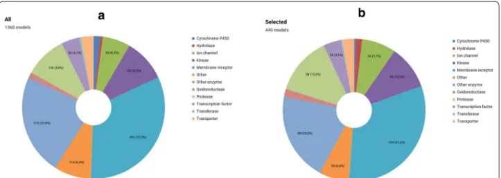
models, further referred to as point prediction models, out of the initial set of 1360 models were considered to be reliable and were used for the construction of the rv-QAFFP fingerprint (Additional file 1). The comparison of the representation of target classes between 1360 and 440 models (Fig. 2) shows that the assay space of 1360 models is evenly represented in 440 assays.
The QAFFP fingerprint of an unknown compound is obtained from the predictions of point prediction mod-els applied on this compound. However, if the compound lies outside the Applicability Domain (AD) of the point prediction model, its biological activity might not be pre-dicted reliably [70, 71]. Thus, it is important to estimate model AD. In the present work, the AD was estimated using the Conformal Prediction (CP) framework [53, 56].
A conformal predictor is the type of a confidence dictor that outputs, in contrast to a single value, a pre-diction interval with a guaranteed maximum error rate corresponding to a user-defined confidence level1−ε , where ε is called a significance level. For example, for a conformal regression model at 90% confidence level (i.e., at 10% significance level), at least 90% of all gener-ated prediction intervals contain the correct value (i.e., no more than 10% of the actual values are outside the prediction interval). For each new compound, the non-conformity score (measure) α is calculated. The
noncon-formity score is the way of measuring how similar a new compound is to the training set compounds and it is defined as α = |yi−yi|
i where yi is the observed
bioactiv-ity value, yi is the predicted bioactivity value and i is the
scaling factor of the prediction interval. In the present work, a separate RF model, an error prediction model, was trained to predict the residual ρi (i.e., the difference
between the measured bioactivity and bioactivity pre-dicted by the point prediction model), and this value was
used as the scaling factor i . The Conformal Predictor is
then relating and ranking nonconformity scores of com-pounds to be predicted to scores of previously experi-mentally tested compounds. This is done by calculating a p-value (not to be confused with a p-value in statisti-cal analysis), which is the fraction of existing compounds with nonconformity scores α smaller than is that of the new compound. If this fraction is small, the new com-pound is very non-conforming, i.e. rather different from previous compounds in the model, and it will hence have larger associated prediction ranges.
In this work, inductive conformal prediction (ICP) [72] was employed. In ICP, the training set is randomly divided into a “proper” training set and a “calibration” set. The model is trained using the proper training set and the calibration set is used to generate nonconformity scores
α . The disadvantage of ICP is that it requires more data
because the calibration set instances must not be used to train the model. Therefore, we utilized cross-confor-mal prediction (CCP) [73] in which data are, similarly to cross-validation, divided in k folds (k equals 10 in the present work) and hence all training data are used as the training as well as the calibration set in turn.
b‑QAFFP fingerprint construction
A standard molecular representation used in similarity searching are binary fingerprints [74]. To compare the performance of rv-QAFFP with ECFP4 binary fingerprint [2], which has been established as a well-performing benchmark method in several previous studies [75–77], rv-QAFFP was converted to a binary form, b-QAFFP, using an activity cutoff and taking into account model AD. The predicted value was considered to lie within model AD if, at the given confidence level, the width of the prediction interval does not exceed a threshold the
value of which was optimized. In b-QAFFP, all predicted values that lie above the activity cutoff and which are, at the same time, within model AD, were encoded as ones. All values that lie below the affinity cutoff but are still within model AD were encoded as zeros. Also, if the pre-diction lies outside model AD, the value was set to zero assuming that a compound is more likely to be inactive than active, similarly to what was reported in several pre-vious studies [1, 29, 78].
QAFFP performance assessment
The value of the QAFFP fingerprint was demonstrated for three common chemoinformatics applications: simi-larity searching, biological activity classification and scaffold hopping. In addition, the accompanying paper [REFERENCE GOES HERE] describes the application of QAFFP fingerprint in regression setting for the predic-tion of compound in vitro potency.
1) Similarity searching. In similarity searching, new potentially active compounds are identified by cal-culating their structural similarity [79, 80] to already known actives. This approach is based on a similar property relationship which states that structurally similar compounds possess similar properties [81]. Similarity searching is suitable if just one active com-pound is known. In similarity searching task, only the performance of the b-QAFFP fingerprint was evalu-ated.
2) Biological activity classification. In a biological activ-ity classification, known actives and inactives are taken as an input to build a classification model that is used to classify unknown compounds. Typically, machine learning approaches are used as classifiers [82, 83]. Machine learning classification approaches are suitable if several actives are available. In a bio-logical activity classification, the performance of both the rv-QAFFP and b-QAFFP fingerprints was evalu-ated.
3) Scaffold hopping. The aim of scaffold hopping is to discover active compounds that contain entirely new chemotypes [84–86]. The scaffold hopping potential was evaluated both for the rv-QAFFP and b-QAFFP fingerprints.
QAFFP fingerprint performance was assessed by two quality measures, AUC and EF5, the combination of which gives a good idea about the ability of the method to separate true positives from false positives [87]. AUC is the area under the ROC curve and it quantifies the gen-eral ability of a method to discriminate between actives and inactives [88]. AUC equals to the probability that a classifier will rank a randomly chosen positive instance
higher than a randomly chosen negative example. How-ever, AUC is not sufficiently sensitive to an early recog-nition [89], meaning that it does not prioritize models that place actives earlier in the ranked list of compounds. Thus, AUC was supplemented by the enrichment factor EF that explicitly measures the early recognition [89, 90]. EF is defined [91] as
where χ% is the fraction of the sorted dataset EF is
calcu-lated for, Pχ% is the number of actives in this fraction and
Nχ% is the number of all molecules in this fraction, Ptotal
is the number of actives in the data set and Ntotal the
number of all molecules in the data set. A method that is superior to a random selection of compounds returns EF > 1. In this study, EF at top 5% ( χ= 0.05) of the sorted data set, abbreviated as EF5, was calculated.
QAFFP performance was compared to 1024 bits long Morgan2 fingerprint which is the equivalent of the ECFP4 fingerprint [2]. The ECFP4 fingerprint was chosen as a baseline for comparisons because of its high retrieval rates in various benchmarking studies [76, 92]. Differ-ences in the performance between QAFFP and Morgan2 fingerprints were assessed by a one-sided exact Wilcoxon paired signed-rank test (a nonparametric alternative for the paired t-test) implemented in the R package coin [93, 94]. The effect size was assessed as a two-sided 95% con-fidence interval of the average difference of the criterion (AUC or EF5) between QAFFP and Morgan2 constructed by two-sided exact Wilcoxon signed-rank procedure.
Similarity searching
The performance of the b-QAFFP fingerprint in simi-larity searching was assessed using the open-source benchmarking platform developed by Riniker et al. [90, 95]. The platform contains the lists of actives and inac-tives gathered from three different data collections (DUD [96], MUV [97] and ChEMBL [50, 51] subset proposed by Heikamp and Bajorath [98]), lists of predefined training sets, lists of randomly selected query molecules and the Python code needed to perform the evaluation. The avail-ability of predefined training and test (i.e. query) mole-cules enables the easy reproduction of virtual screening experiments and the comparison of their results.
Two distinct data sets (Additional file 2) that simulate two following use cases are provided within the current version of the platform [95]:
1) Use case: a small set of diverse actives from a high-throughput screen is available. For this use case, heterogeneous data sets (further referred to as HET EF(χ%)=
data sets, “data sets I” in the original publication [95]) consisting of 69 sets were assembled from the follow-ing three sources: 16 Maximum Unbiased Validation (MUV) data sets [97], 3 data sets from the Direc-tory of Useful Decoys (DUD) [99], and 50 data sets extracted from ChEMBL [98].
2) Use case: a small set of related actives, i.e. compounds sharing one or two common scaffolds, from a publi-cation or patent is available. For this use case, homo-geneous data sets (further referred to as HOM data sets, “data sets II” in the original publication [95]) consisting of 37 sets were extracted from medicinal-chemistry papers that typically include data on one or two chemical series.
Both HET and HOM data sets contain assays that are also present in the QAFFP fingerprint and these were, thus, removed from the QAFFP fingerprint. Namely, out of 69 HET targets, 44 targets that correspond to 56 QAFFP assays are present in the QAFFP fingerprint (Additional file 2) which becomes, upon their removal, 384 bits long. Similarly, out of 37 HOM targets, 27 targets that corre-spond to 38 QAFFP assays are present in the QAFFP fin-gerprint (Additional file 2) which becomes, upon their removal, 402 bits long.
For each target of three data-set collections (MUV, DUD, ChEMBL), two compound lists are provided within the benchmarking platform, one for actives and one for inac-tives. For HET data sets, the VS experiment was repeated 50 times for each target, with different randomly selected training sets. To ensure the reproducibility of the results, the precalculated training sets are provided as the part of the benchmarking platform. In our case, each training set consisted of 10 actives (further referred to as query mol-ecules) and of 20% of randomly selected inactives. The remaining actives and inactives formed the test set. For each molecule in the test set, its similarity to query mol-ecules was calculated and only the highest similarity value was considered, corresponding to the MAX fusion rule [100]. The whole test set was then sorted by the decreas-ing similarity and AUC and EF5 were calculated from this ranked list.
For HOM data sets, the VS experiment was performed once for each paper using, as the training set, all actives from the paper and 10% of the inactives. The test set con-sisted of 99 actives from the benchmarking data set for the same target and the rest of the inactives.
The similarity between molecules was evaluated by the Rogot-Goldberg index sRG [101]
sRG=
a
2a+b+c+
d
2d+b+c
where a is the number of bits set to 1 in both objects, d is the number of bits set to 0 in both objects, b is the number of cases in which bits in the first objects are set to 1 and bits in the second object are, at the same time, set to 0, and c is the number of events in which bits in the first objects are set to 0 and bits in the second object are, at the same time, set to 1. The Rogot-Goldberg index represents an efficient alternative [102] to the commonly used Tanimoto index, however, it takes into account not only bits set to 1, but also bits set to 0. For the b-QAFFP fingerprint, the Rogot-Goldberg index is more realistic measure than the Tanimoto index because the informa-tion at which targets the compound is active is equally important as the information at which targets it is inactive.
To compare the performance of the b-QAFFP and Morgan2 fingerprints, both types of fingerprints were calculated for HET and HOM data sets. The affinity cutoffs of 5 (i.e., 10 µM), 6 (i.e., 1 µM), 7 (i.e., 100 nM) and 8 (i.e., 10 nM) were used for the construction of the b-QAFFP fingerprint. Model AD was estimated using conformal prediction, but the case of not using AD was also considered. An ICP was used with the confidence level of 90% and the maximum interval width, that distin-guishes whether the prediction is reliable enough, was set to 4.0 (i.e., predicted value ± 2.0). For every data set and every type of fingerprint, a separate model was trained and its performance was assessed by calculating the AUC and EF5 values for the test set.
Biological activity classification
Both HET and HOM sets are highly imbalanced with a considerably higher amount of inactives (e.g., MUV data sets contain 30 actives and 15,000 inactives, see Addi-tional file 2), which limits their utility for the training of a classification model. Thus, new data sets, further referred to as the CLASS data sets, were constructed from 920 assays that were not used for QAFFP construction. The CLASS data sets were selected using the following crite-ria: (1) compounds with a potency ≤ 5 were considered as inactive, compounds with a potency ≥ 6 as active, (2) for every CLASS data set (assay), more than 60 inac-tives and more than 60 acinac-tives must be available (3) only assays that share no more than 10% of ligands with any of QAFFP assays were included in the CLASS data sets. The CLASS data sets consist of 23 assays (21 IC50 and 2 EC50) covering 23 targets (Additional file 3).
constructed using several affinity cutoffs (5 (i.e., 10 µM), 6 (i.e., 1 µM), 7 (i.e., 100 nM) and 8 (i.e., 10 nM)) consid-ering or not considconsid-ering the AD that was estimated by an ICP using the confidence level of 90% and the maximum interval width was set to 4.0 (i.e., predicted value ± 2.0). All compounds lying outside the AD were substituted with zeros.
In the biological activity classification task, the CLASS data sets were used to train RF models to classify ligands as active or inactive. Because some CLASS data sets are imbalanced (Additional file 3), a balanced RF model [103] from the imbalanced-learn Python package [79] was trained. Each RF model consisted of 100 trees [53, 63, 64] and GINI index was used as a purity criterion to split a node. Ligands were encoded by the Morgan2 (1024 bits long), rv-QAFFP and b-QAFFP (both 440 bits long) fin-gerprints. fivefold cross-validation was used to evaluate model performance. Each cross-validation was repeated 10-times and final results were averaged over all repeti-tions and all splits.
Scaffold hopping
Scaffold hopping was benchmarked using the CLASS data sets (Additional file 4) with one set removed (ChEMBL ID: CHEMBL5313) as it did not contain enough scaffolds. Ligands were encoded by the Morgan2 (1024 bits long), rv-QAFFP and b-QAFFP (both 440 bits long) fingerprints. The following settings were used to construct the rv-QAFFP and b-QAFFP fingerprints:
1) rv-QAFFP—RF models were trained on raw data considering or not considering model AD estimated by an ICP. At the confidence level of 90%, if the pre-diction interval width was larger than ± 2.0, the pre-diction was considered unreliable and it was replaced by an average of all reliably predicted affinities. 2) b-QAFFP—the affinity cutoffs of 5 (i.e., 10 µM), 6
(i.e., 1 µM), 7 (i.e., 100 nM) and 8 (i.e., 10 nM) were used for the construction of the b-QAFFP finger-print. Model AD was estimated by ICP, but the case of not using AD was also considered. An ICP was used with the confidence level of 90% and with the maximum interval width of ± 2.0. Ligands lying out-side model AD were conout-sidered to be inactive (i.e., corresponding bits were set to 0).
For each ligand, its cyclic skeleton (CSK) [104] was gen-erated. The CSK, also known as a graph framework [105], is derived from the Bemis and Murcko (BM) scaffold [105] by converting all heteroatoms to carbon and set-ting all bond orders to 1. Compound was considered to be active if the negative decadic logarithm of its potency was higher than 6. The CSKs of all active compounds
in a given assay are further referred to as active CSKs (ACSKs). In addition, active CSKs with at least five active compounds are further referred to as rich active CSKs (RACSKs). For the given assay, the training set was formed by compounds from one RACSK plus all inactive compounds. The test set then consisted of all remain-ing active compounds. Thus, the number of trainremain-ing sets for each assay equals to the number of its RACSKs (Additional file 4). Using each training set, a balanced RF model [79, 103] was constructed and applied on the test set. Compounds in the test set were classified either as active or as inactive using the probability threshold of 0.5. For each classified active, its CSK was retrieved and the number of unique CSKs, summed over all training data sets, was calculated for each assay. The scaffold hopping potential was assessed for the Morgan2, rv-QAFFP and b-QAFFP fingerprints. In addition, ACSKs retrieved using both rv- and b-QAFFP fingerprints were pooled and reported as rv+b-QAFFP.
Results and discussion
Data statistics
440 QSAR models used for the QAFFP construction were built using 256 IC50, 137 Ki, 37 EC50 and 10 Kd assays that cover 376 distinct molecular targets; i.e. 64 targets were modeled with more than one assay. However, these “duplicates” are not redundant as the maximum Pearson correlation coefficient between two assays belonging to the same target was only 0.53. 376 targets originate from 34 organisms (Additional file 1), a majority comes from human (254 targets) followed by rat (45 targets) and mouse (18 targets).
Performance of b‑QAFFP fingerprint in similarity searching The results of the evaluation of various approaches for the construction of the b-QAFFP fingerprint are given in the Table 1 for HET data sets, and in the Table 2 for HOM data sets. Further details can be found in the Addi-tional files 5 and 6, Figs. 1 and 2.
The Tables 1 and 2 show that the best setting for the construction of the b-QFFP fingerprint is to estimate the AD with an ICP and to use the affinity cutoff of 5 (i.e., 10 µM). While at this setting the b-QAFFP fingerprint yields statistically significantly better AUC both for the HET and HOM data sets (verified by the one-sided exact Wilcoxon signed-rank test with the p-value for alter-native hypothesis Morgan2 < QAFFP being p-value =
0.21 for two-sided alternative Morgan2 ≠ QAFFP). The corresponding nonparametric 95% confidence intervals reveal that the average excess of b-QAFFP’s AUC over Morgan2’s AUC can be expected in the range from 0.12 to 0.49 for the HET data sets and from 0.58 to 0.12 for the HOM data sets. On the other hand, the 95% non-parametric confidence interval for the average excess of Morgan2’s EF5 over b-QAFFP’s EF5 shows the effect size ranging from 0.28 to 0.69 for the HET sets. The analy-sis of nonparametric 95% confidence intervals for dif-ferences between two fingerprints shows, that though b-QAFFP yields significantly better values than Morgan2 for some measures and vice versa, the effect size is rela-tively small. Thus, it may be concluded that the b-QAFFP and Morgan2 fingerprints they provide comparable results in similarity searching.
Performance of b‑QAFFP and rv‑QAFFP fingerprints in biological activity classification
For every of the 23 CLASS data sets and for every type of fingerprint, a separate RF model was trained and its performance was assessed by calculating the AUC and EF5 for the test set. In addition, rv-QAFFP models were trained using both raw and Z-standardized data (i.e., all data points were converted to their Z-values), but no significant differences between these two approaches were identified. Average value for each quality measure, together with its standard error of the mean, is given in
the Table 3. Further details can be found in the Addi-tional files 6 and 7, Figs. 3 and 4.
The highest rv-QAFFP’s AUC is achieved if the rv-QAFFP fingerprint is constructed from models trained on raw data without regard to their ADs. The difference between considering and not considering the AD lies in a way data points outside the AD are treated. When the AD is taken into account, these data points are imputed by the mean over all reliably predicted affinities. If the AD is not considered, these data points are filled in by pre-dicted affinities, though estimated with less confidence.
The recommended settings for b-QAFFP fingerprint construction are same as those identified for similar-ity searching, i.e. to estimate the AD with an ICP and to use the affinity cutoff of 5 (i.e., 10 µM). At these set-tings, both b-QAFFP and rv-QAFFP fingerprints per-form, in terms of AUC , significantly worse than the Morgan2 fingerprint (p-value of the signed-ranked paired test for alternative Morgan2 > QAFFP is p-value
= 3.58e−07 for both b-QAFFP and rv-QAFFP). The average deficit of b-QAFFP AUC compared to Morgan2 AUC can be expected in the range 0.01–0.03 (with 95% confidence) and the average deficit of rv-QAFFP AUC to Morgan2 AUC in the range 0.01–0.02 (with 95% con-fidence). However, these differences can be considered as small, compared to the average AUC value of ~ 0.86. In terms of EF5, no statistically significant differences were detected between the Morgan2, b-QAFFP and
Table 1 The comparison of the performance of the Morgan2 (ECFP4) and b-QAFFP fingerprints for similarity searching for 69 HET data sets
Model AD was estimated by an ICP. Affinities predicted to lie outside model AD were encoded by zeros. Various affinity cutoffs were used to construct the b-QAFFP fingerprint. Best results are shown in a column in italic. Data shown are averages over all HET data sets with their standard errors of the mean. The b-QAFFP fingerprint is 384 bits long
FP Morgan2 b‑QAFFP
AD – No Yes
Cutoff – 5 6 7 8 5 6 7 8
AUC 0.66 ± 0.01 0.63 ± 0.01 0.63 ± 0.01 0.65 ± 0.01 0.58 ± 0.01 0.70 ± 0.01 0.62 ± 0.01 0.63 ± 0.01 0.56 ± 0.01 EF5 6.41 ± 0.40 3.67 ± 0.25 4.52 ± 0.33 4.50 ± 0.30 2.27 ± 0.16 5.82 ± 0.34 4.65 ± 0.32 3.97 ± 0.26 1.76 ± 0.12
Table 2 The comparison of the performance of the Morgan2 (ECFP4) and b-QAFFP fingerprints for similarity searching for 37 HOM data sets
Model AD was estimated by an ICP. Affinities predicted to lie outside model AD were encoded by zeros. Various affinity cutoffs were used to construct the b-QAFFP fingerprint. Best results are shown in a column in italic. Data shown are averages over all HOM data sets with their standard errors of the mean. The b-QAFFP fingerprint is 402 bits long
FP Morgan2 b‑QAFFP
AD – No Yes
Cutoff – 5 6 7 8 5 6 7 8
rv-QAFFP fingerprints. Therefore, the performance of the QAFFP fingerprints can be considered comparable to that of the Morgan2 fingerprint also for biological activ-ity classification.
Performance of b‑QAFFP and rv‑QAFFP fingerprints in scaffold hopping
For every of the 22 CLASS data sets (one CLASS data set was not used as it contained no RACSK) and for every type of fingerprint, a separate RF model was trained and its performance was assessed by calculating the average number of ACSKs per an assay (Table 4).
Table 4 reveals that for both rv-QAFFP and b-QAFFP there are no differences in the performance whether AD is considered or not. The average number of recovered ACSKs is lower for rv-QAFFP compared
to b-QFFP. For b-QAFFP, the results are pretty sta-ble for thresholds of 5, 6 and 7. Only for threshold 8, a significant increase in the average number of recov-ered ACSKs can be observed. Threshold 8 means that only very potent molecules (< 10 nM) are considered as active, at this threshold b-QAFFP bit density dramati-cally drops (Table 5) and data become too sparse. For sparse data, it’s very likely that for some RF node the bootstrapped sample and the random subset of features will play along to produce an invariant feature space. This will influence RF predictions and, thus, threshold 8 can be considered as an extreme case.
QAFFP scaffold hopping potential was assessed for rv-QAFFP constructed from raw data without con-sidering model AD and for b-QAFFP using affinity threshold of 5 and estimating model AD by an ICP sub-stituting missing values (unreliable predictions with interval wider than ± 2.0 at the confidence level of 90%) by zeros. These settings, though suboptimal, are con-sistent with settings for similarity searching (Tables 1 and 2) and biological activity classification (Table 3).
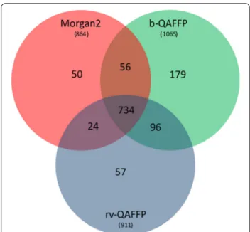
Out of 1749 existing ACSKs from 22 CLASS data sets, the Morgan2 fingerprint revealed 864 (49%) and the rv-QAFFP fingerprint 911 ACSKs (52%) (Figs. 3, 4, Additional file 4). The differences between Morgan2 and rv-QAFFP (Table 6) are not statistically significant (p-value of two sided Wilcoxon signed-rank paired test is 0.11). On the other hand, the b-QAFFP fingerprint, that unveiled 1065 (61%) ACSKs, performed significantly better (p-value = 1.43e−04 for alternative b-QAFFP > Morgan2 using Wilcoxon signed-rank paired test) than the Morgan2 fingerprint. The highest number of ACSKs (1146. i.e. 66%) was identified when ACSKs found by the rv-QAFFP and b-QAFFP were joined together (further denoted as rv+b-QAFFP). This combination works sta-tistically significantly better than the b-QAFFP finger-print alone (p-value = 1.43e−04 for alternative b-QAFFP > rv+b-QAFFP using Wilcoxon signed-rank paired test).
Table 3 The comparison of the performance of the Morgan2 (ECFP4), rv-QAFFP and b-QAFFP fingerprints for biological activity classification of 23 CLASS data sets
Model AD was estimated by an ICP with the confidence level of 90%. rv-QAFFP models were trained using raw data. Considering AD for rv-QAFFP means that if the prediction interval width was larger than ± 2.0, the prediction was regarded unreliable and was replaced by the average of all reliably predicted affinities. Various affinity cutoffs were used to construct the b-QAFFP fingerprint. Affinities predicted to lie outside model AD were encoded by zeros. Best results are shown in columns in italic. Data shown are averages over all CLASS data sets with their standard errors of the mean. Both rv-QAFFP and b-QAFFP fingerprints are 440 bits long FP Morgan2 rv‑QAFFP b‑QAFFP
AD – No Yes No Yes
Cutoff – – – 5 6 7 8 5 6 7 8
AUC 0.87 ± 0.01 0.86 ± 0.01 0.86 ± 0.02 0.83 ± 0.01 0.85 ± 0.01 0.84 ± 0.02 0.77 ± 0.01 0.85 ±0.02 0.85 ± 0.02 0.83 ± 0.02 0.73 ± 0.01 EF5 2.16 ± 0.16 2.08 ±0.14 2.08 ± 0.13 2.03 ± 0.13 2.09 ± 0.14 2.08 ± 0.14 1.89 ± 0.11 2.10 ±0.14 2.08 ± 0.14 2.04 ± 0.13 1.78 ± 0.10
Thus, it may be concluded that while the Morgan2 and rv-QAFFP fingerprints exhibit similarly low scaf-fold hopping potential, the b-QAFFP fingerprint is better by ca 10%. The highest number of ACSKs was revealed when ACSKs from both rv-QAFFP and b-QAFFP fingerprints were joined together; this com-bination yielded 17% more ACSKs than the Morgan2 fingerprint.
Conclusions
constructed by the binarization of the rv-QAFFP finger-print. The following settings are recommended for the construction of the rv-QAFFP and b-QAFFP fingerprints:
• rv-QAFFP—use predicted bioactivities (i.e., it is not necessary to Z-standardize them) without consid-ering model AD.
• b-QAFFP—to binarize rv-QAFFP values, use the affinity threshold of 5 on the –log scale, estimate model AD by an ICP, substitute missing values (unreliable predictions with interval wider than
± 2.0 at the confidence level of 90%) by zeros.
We would like to stress, that though there exist many tunable settings in QAFFP construction pipeline, our aim was not to optimize each of them for every con-ceivable application. That would lead to lots of different
settings for different use cases which would be rather confusing for the end user. Instead, we decided to pro-pose such QAFFP setting that is robust enough and yields constantly reasonable results. We believe that our published recommendations for the construction of rv- and b-QAFFP fingerprints meet these requirements.
The performance of both QAFFP fingerprints was assessed in three cheminformatics tasks: similarity searching, bioactivity classification and scaffold hop-ping. In all tasks, the QAFFP fingerprints were com-pared to 1024 bits long Morgan2 fingerprint (Morgan fingerprint with the radius of 2, an equivalent to the ECFP4 fingerprint) using non-parametric Wilcoxon paired signed-rank test. It was found that the perfor-mance of both rv-QAFFP and b-QAFFP fingerprints is similar to that of the Morgan2 (ECFP4) fingerprint in similarity searching and bioactivity classification. How-ever, compared to the Morgan2 fingerprint, the QAFFP fingerprints were able to retrieve significantly higher number of new scaffolds. These findings are rather encouraging given that (i) the QAFFP fingerprints are much shorter, (ii) the QAFFP fingerprints are defined on a purely data-driven fashion, without selecting the targets following biological reasons, and (iii) the mod-els from which the QAFFP fingerprints are derived are far from perfect as their quality is influenced by, for example, QSAR modeling errors [106, 107], experi-mental errors in publicly available data [108–110], data curation errors [68, 111] or data imputation noise. On
Table 4 The average number of ACSKs per an assay (and its standard error of the mean SEM) in 22 CLASS sets revealed by the Morgan2, rv-QAFFP and b-QAFFP fingerprints
Model AD was estimated by an ICP with the confidence level of 90%. rv-QAFFP models were trained using raw data. Considering AD for rv-QAFFP means that if the prediction interval width was larger than ± 2.0, the prediction was regarded unreliable and was replaced by the average of all reliably predicted affinities. Various affinity cutoffs were used to construct the b-QAFFP fingerprint. Affinities predicted to lie outside model AD were encoded by zeros. Data shown are averages over 22 CLASS data sets with their standard errors of the mean (SEM). Both rv-QAFFP and b-QAFFP fingerprints are 440 bits long. The recommended settings are shown in columns in italic
FP Morgan2 rv‑QAFFP b‑QAFFP
AD No Yes No Yes
Cutoff – – – 5 6 7 8 5 6 7 8
Average 39.27 41.41 41.45 48.40 47.80 48.89 66.14 48.41 47.89 48.54 67.58 SEM 8.25 8.51 8.68 10.26 10.47 11.18 16.02 10.37 10.54 10.88 16.84
Table 5 The average number of ON bits in b-QAFFPs calculated for HET set compounds
Model AD was estimated by an ICP with the confidence level of 90% and the maximum interval width, that distinguishes whether the prediction is reliable enough, was set to ± 2.0. Affinities predicted to lie outside model AD were encoded by zeros. b-QAFFP is 440 bits long
no AD AD
Cutoff 5 6 7 8 5 6 7 8
Average [%] 92.5 53.5 14.5 1.6 71.1 39.4 10.4 1.2
Average [count] 407 235 64 7 313 174 46 5
Table 6 The average number of ACSKs per an assay revealed by the Morgan2, rv-QAFFP and b-QAFFP fingerprints in 22 CLASS sets
In addition, the union of ACSKs revealed by both rv-QAFFP and b-QAFFP is reported. Averages are shown together with their standard errors of the mean. Additional file 4 contains detailed information about the number of revealed ACSKs for individual assays
Morgan2 rv‑QAFFP b‑QAFFP rv+b‑QAFFP
Average # of
the other hand, QAFFP fingerprint is de facto a set of transformed Morgan fingerprints and it, thus, implic-itly considers the structure of compounds. For this rea-son, two structurally similar compounds will show a similar predicted QAFFP profile and possible “activity cliffs” [112, 113] will not be identified.
To conclude, despite the fact that the QAFFP finger-prints are defined on a purely data-driven fashion and that underlying QSAR models rely solely on public data, we have demonstrated that large-scale QSAR modeling [114] is a promising method for the construction of affinity fingerprints. Though affinity fingerprints are inherently noisy, a signal-to-noise ratio is high enough to enable the discovery of bioactive molecules based on biological similarity rather than chemical similarity. In the future, we plan to optimize the composition of the QAFFP fin-gerprint [115] and to use more biology-informed criteria (e.g., bioactivity data on cancer-related targets are likely to provide high predictive power to find hits eliciting anticancer activity). Future studies will also be needed to investigate the utility of both binary and real-valued QAFFP fingerprints for ligand and target clustering or to evaluate the utility of the QAFFP fingerprint for com-mon computational drug design tasks, including diversity selection, hit expansion, target identification, drug repur-posing, and the prediction of adverse side effect.
Supplementary information
Supplementary information accompanies this paper at https ://doi. org/10.1186/s1332 1‑020‑00443 ‑6.
Additional file 1. QAFFP construction. Statistics (ligand count and quality criteria q2 and R′02 ) of all 1360 trained models. Each model is given by the target ChEMBL ID and by an activity type (Ki, Kd, IC50 or EC50). 440 models used to construct the QAFFP fingerprint highlighted in green. Ligand data of 440 models (given as ligand ChEMBL ID, SMILES, activity type and activity value).
Additional file 2. Similarity searching task. The list of HET and HOM data sets including the number of actives and inactives.
Additional file 3. Biological activity classification task. The list of CLASS data sets including the number of actives and inactives.
Additional file 4. Scaffold hopping task. The list of targets used for scaf‑ fold hopping potential assessment, the number of ACSKs and RACSKs and the number of ACSKs retrieved using the Morgan2, b‑QAFFP and rv‑QAFFP fingerprints and the combination rv+b‑QAFFP.
Additional file 5. Similarity searching task. Average values of AUC and EF5 for individual sets in the HET and HOM data sets obtained using various settings (affinity cutoffs of 5‑8, AD estimation turned on and off ) for the construction of the b‑QAFFP fingerprint.
Additional file 6. Similarity searching and biological activity classifica‑ tion tasks. Plots showing the performance of the QAFFP and Morgan2 fingerprints.
Additional file 7. Biological activity classification task. Average values of AUC and EF5 for individual sets in the CLASS data sets obtained using vari‑ ous settings (affinity cutoffs of 5‑8, AD estimation turned on and off ) for the construction of the b‑QAFFP and rv‑QAFFP fingerprints.
Abbreviations
ACSK: Active cyclic skeleton; AD: Applicability domain; AUC : Area under the ROC curve; BAF: Bayes affinity fingerprint; BM scaffold: Bemis and Murcko scaffold; b‑QAFFP: Binary; QAFFP CCP: Cross‑conformal prediction; CLASS: Biological activity classification data sets; CP: Conformal prediction; CSK: Cyclic skeleton; DUD: Directory of useful decoys; ECFP: Extended connectiv‑ ity fingerprint; EF: Enrichment factor; FN: False negatives; FP: False positives; HET: Heterogeneous data sets; HOM: Homogeneous data sets; HTS: High throughput screening; HTSFP: HTS fingerprint; ICP: Inductive conformal prediction; Morgan2: Morgan fingerprint with the radius of 2; MUV: Maximum Unbiased Validation data sets; QAFFP: QSAR affinity fingerprint; QSAR: Quan‑ titative structure‑activity relationship; RACSK: Rich active cyclic skeleton; ROC: Receiver operating characteristic; Sen: Sensitivity; Spe: Specificity; TN: True negatives; TP: True positives; VS: Virtual screening.
Acknowledgements
Computational resources were provided by the CESNET LM2015042 and the CERIT Scientific Cloud LM2015085, provided under the programme “Projects of Large Research, Development, and Innovations Infrastructures”.
Authors’ contributions
CŠ, IT and DS conceived the study. CŠ, IC‑C, WD and GJPvW were responsible for method development, implementation and validation. PK was responsible for statistical data analysis. DS supervised the study. DS, CŠ and IC‑C wrote the manuscript. IVT, GJPvW, AB and PK edited the manuscript. All authors read and approved the final manuscript.
Funding
This work was supported by the Ministry of Education, Youth and Sports of the Czech Republic – project number LM2018130 (C. Š., D. S., W. D.) and by RVO 68378050‑KAV‑NPUI (C. Š., D. S.). This project has received funding from the European Union’s Framework Programme for Research and Innova‑ tion Horizon 2020 (2014–2020) under the Marie Sklodowska‑Curie Grant Agreement No. 703543 (I. C. C.) and FP7 Marie Sklodowska‑Curie ITN project “Environmental Chemoinformatics” (ECO), grant agreement number 238701 (C. Š. and I. V. T.).
Availability of data and materials
The datasets supporting the conclusions of this article are included as addi‑ tional files. The source code with the workflow for the generation of QAFFPs is available from GitHub repository: https ://githu b.com/skuta c/QAFFP s.
Competing interests
The authors declare that they have no competing interests.
Author details
1 CZ‑OPENSCREEN: National Infrastructure for Chemical Biology, Institute
of Molecular Genetics of the ASCR, v. v. i., Vídeňská 1083, 142 20 Prague 4, Czech Republic. 2 Centre for Molecular Informatics, Department of Chem‑
istry, University of Cambridge, Lensfield Road, Cambridge CB2 1EW, UK.
3 CZ‑OPENSCREEN: National Infrastructure for Chemical Biology, Department
of Informatics and Chemistry, Faculty of Chemical Technology, University of Chemistry and Technology Prague, Technická 5, 166 28 Prague, Czech Republic. 4 Department of Mathematics, Faculty of Chemical Engineering,
University of Chemistry and Technology Prague, Technická 5, 166 28 Prague, Czech Republic. 5 Computational Drug Discovery, Drug Discovery and Safety,
LACDR, Leiden University, Einsteinweg 55, 2333 CC Leiden, The Netherlands.
6 Helmholtz Zentrum Muenchen – German Research Center for Environmental
Health (GmbH) and BIGCHEM GmbH, Ingolstaedter Landstrasse 1, 85764 Neu‑ herberg, Germany.
Received: 7 August 2019 Accepted: 16 May 2020
References
1. Tanrikulu Y, Kruger B, Proschak E (2013) The holistic integration of virtual screening in drug discovery. Drug Discov Today 18(7–8):358–364 2. Rogers D, Hahn M (2010) Extended‑connectivity fingerprints. J Chem
3. Consonni V, Todeschini R (2000) Handbook of molecular descriptors. Wiley‑VCH, New York
4. Wassermann AM, Lounkine E, Davies JW, Glick M, Camargo LM (2015) The opportunities of mining historical and collective data in drug discovery. Drug Discov Today 20(4):422–434
5. Paricharak S, Mendez‑Lucio O, Chavan Ravindranath A, Bender A, Ijzerman AP, van Westen GJ (2016) Data‑driven approaches used for compound library design, hit triage and bioactivity modeling in high‑ throughput screening. Brief Bioinform 19(2):277–285
6. Shoemaker RH (2006) The NCI60 human tumour cell line anticancer drug screen. Nat Rev Cancer 6(10):813–823
7. Paull KD, Shoemaker RH, Hodes L, Monks A, Scudiero DA, Rubinstein L, Plowman J, Boyd MR (1989) Display and analysis of patterns of differential activity of drugs against human tumor cell lines: develop‑ ment of mean graph and COMPARE algorithm. J Natl Cancer Inst 81(14):1088–1092
8. Zaharevitz DW, Holbeck SL, Bowerman C, Svetlik PA (2002) COMPARE: a web accessible tool for investigating mechanisms of cell growth inhibi‑ tion. J Mol Graph Model 20(4):297–303
9. Weinstein JN, Kohn KW, Grever MR, Viswanadhan VN, Rubinstein LV, Monks AP, Scudiero DA, Welch L, Koutsoukos AD, Chiausa AJ et al (1992) Neural computing in cancer drug development: predicting mechanism of action. Science 258(5081):447–451
10. Weinstein JN, Myers TG, O’Connor PM, Friend SH, Fornace AJ Jr, Kohn KW, Fojo T, Bates SE, Rubinstein LV, Anderson NL et al (1997) An information‑intensive approach to the molecular pharmacology of cancer. Science 275(5298):343–349
11. Kauvar LM, Higgins DL, Villar HO, Sportsman JR, Engqvist‑Goldstein A, Bukar R, Bauer KE, Dilley H, Rocke DM (1995) Predicting ligand binding to proteins by affinity fingerprinting. Chem Biol 2(2):107–118 12. Fliri AF, Loging WT, Thadeio PF, Volkmann RA (2005) Biological spectra
analysis: linking biological activity profiles to molecular structure. Proc Natl Acad Sci USA 102(2):261–266
13. Fliri AF, Loging WT, Thadeio PF, Volkmann RA (2005) Biospectra analysis: model proteome characterizations for linking molecular structure and biological response. J Med Chem 48(22):6918–6925
14. Haggarty SJ, Clemons PA, Schreiber SL (2003) Chemical genomic profil‑ ing of biological networks using graph theory and combinations of small molecule perturbations. J Am Chem Soc 125(35):10543–10545 15. Kim YK, Arai MA, Arai T, Lamenzo JO, Dean EF 3rd, Patterson N, Clemons
PA, Schreiber SL (2004) Relationship of stereochemical and skeletal diversity of small molecules to cellular measurement space. J Am Chem Soc 126(45):14740–14745
16. Anzali S, Barnickel G, Cezanne B, Krug M, Filimonov D, Poroikov V (2001) Discriminating between drugs and nondrugs by prediction of activity spectra for substances (PASS). J Med Chem 44(15):2432–2437 17. Poroikov V, Filimonov D, Lagunin A, Gloriozova T, Zakharov A (2007)
PASS: identification of probable targets and mechanisms of toxicity. SAR QSAR Environ Res 18(1–2):101–110
18. Beroza P, Damodaran K, Lum RT (2005) Target‑related affinity profiling: Telik’s lead discovery technology. Curr Top Med Chem 5(4):371–381 19. Hsu N, Cai D, Damodaran K, Gomez RF, Keck JG, Laborde E, Lum
RT, Macke TJ, Martin G, Schow SR et al (2004) Novel cyclooxyge‑ nase‑1 inhibitors discovered using affinity fingerprints. J Med Chem 47(20):4875–4880
20. Wadkins RM, Hyatt JL, Yoon KJ, Morton CL, Lee RE, Damodaran K, Beroza P, Danks MK, Potter PM (2004) Discovery of novel selective inhibitors of human intestinal carboxylesterase for the amelioration of irinotecan‑ induced diarrhea: synthesis, quantitative structure‑activity relationship analysis, and biological activity. Mol Pharmacol 65(6):1336–1343 21. Plouffe D, Brinker A, McNamara C, Henson K, Kato N, Kuhen K, Nagle A,
Adrian F, Matzen JT, Anderson P et al (2008) In silico activity profiling reveals the mechanism of action of antimalarials discovered in a high‑ throughput screen. Proc Natl Acad Sci USA 105(26):9059–9064 22. Petrone PM, Simms B, Nigsch F, Lounkine E, Kutchukian P, Cornett A,
Deng Z, Davies JW, Jenkins JL, Glick M (2012) Rethinking molecular similarity: comparing compounds on the basis of biological activity. ACS Chem Biol 7(8):1399–1409
23. Dancik V, Carrel H, Bodycombe NE, Seiler KP, Fomina‑Yadlin D, Kubicek ST, Hartwell K, Shamji AF, Wagner BK, Clemons PA (2014) Connecting
small molecules with similar assay performance profiles leads to new biological hypotheses. J Biomol Screen 19(5):771–781
24. Petrone PM, Wassermann AM, Lounkine E, Kutchukian P, Simms B, Jenkins J, Selzer P, Glick M (2013) Biodiversity of small molecules– a new perspective in screening set selection. Drug Discov Today. 18(13–14):674–680
25. Wassermann AM, Lounkine E, Urban L, Whitebread S, Chen S, Hughes K, Guo H, Kutlina E, Fekete A, Klumpp M et al (2014) A screening pattern recognition method finds new and divergent targets for drugs and natural products. ACS Chem Biol 9(7):1622–1631
26. Cortes Cabrera A, Lucena‑Agell D, Redondo‑Horcajo M, Barasoain I, Diaz JF, Fasching B, Petrone PM (2016) Aggregated compound biological signatures facilitate phenotypic drug discovery and target elucidation. ACS Chem Biol 11(11):3024–3034
27. Maciejewski M, Wassermann AM, Glick M, Lounkine E (2015) Experi‑ mental design strategy: weak reinforcement leads to increased hit rates and enhanced chemical diversity. J Chem Inf Model 55(5):956–962 28. Paricharak S, Ijzerman AP, Bender A, Nigsch F (2016) Analysis of iterative
screening with stepwise compound selection based on Novartis in‑ house HTS data. ACS Chem Biol 11(5):1255–1264
29. Riniker S, Wang Y, Jenkins JL, Landrum GA (2014) Using information from historical high‑throughput screens to predict active compounds. J Chem Inf Model 54(7):1880–1891
30. Wang Y, Bryant SH, Cheng T, Wang J, Gindulyte A, Shoemaker BA, Thies‑ sen PA, He S, Zhang J (2017) PubChem BioAssay: 2017 update. Nucleic Acids Res 45(D1):D955–D963
31. Helal KY, Maciejewski M, Gregori‑Puigjane E, Glick M, Wassermann AM (2016) Public domain HTS fingerprints: design and evaluation of com‑ pound bioactivity profiles from PubChem’s Bioassay Repository. J Chem Inf Model 56(2):390–398
32. Briem H, Kuntz ID (1996) Molecular similarity based on DOCK‑gener‑ ated fingerprints. J Med Chem 39(17):3401–3408
33. Coleman RG, Carchia M, Sterling T, Irwin JJ, Shoichet BK (2013) Ligand pose and orientational sampling in molecular docking. PLoS ONE 8(10):e75992
34. Lessel UF, Briem H (2000) Flexsim‑X: a method for the detection of molecules with similar biological activity. J Chem Inf Comput Sci 40(2):246–253
35. Rarey M, Kramer B, Lengauer T, Klebe G (1996) A fast flexible dock‑ ing method using an incremental construction algorithm. J Mol Biol 261(3):470–489
36. Simon Z, Vigh‑Smeller M, Peragovics A, Csukly G, Zahoranszky‑Kohalmi G, Rauscher AA, Jelinek B, Hari P, Bitter I, Malnasi‑Csizmadia A et al (2010) Relating the shape of protein binding sites to binding affinity profiles: is there an association? BMC Struct Biol 10:32
37. Vegner L, Peragovics A, Tombor L, Jelinek B, Czobor P, Bender A, Simon Z, Malnasi‑Csizmadia A (2013) Experimental confirmation of new drug‑ target interactions predicted by Drug Profile Matching. J Med Chem 56(21):8377–8388
38. Peragovics A, Simon Z, Malnasi‑Csizmadia A, Bender A (2016) Modeling polypharmacological profiles by affinity fingerprinting. Curr Pharm Des 22(46):6885–6894
39. Murali S, Hojo S, Tsujishita H, Nakamura H, Fukunishi Y (2007) In‑silico drug screening method based on the protein‑compound affin‑ ity matrix using the factor selection technique. Eur J Med Chem 42(7):966–976
40. Fukunishi Y, Hojo S, Nakamura H (2006) An efficient in silico screening method based on the protein‑compound affinity matrix and its appli‑ cation to the design of a focused library for cytochrome P450 (CYP) ligands. J Chem Inf Model 46(6):2610–2622
41. Bender A, Jenkins JL, Glick M, Deng Z, Nettles JH, Davies JW (2006) “Bayes affinity fingerprints” improve retrieval rates in virtual screening and define orthogonal bioactivity space: when are multitarget drugs a feasible concept? J Chem Inf Model 46(6):2445–2456
42. Cherkasov A, Muratov EN, Fourches D, Varnek A, Baskin II, Cronin M, Dearden J, Gramatica P, Martin YC, Todeschini R et al (2014) QSAR mod‑ eling: where have you been? Where are you going to? J Med Chem 57(12):4977–5010
44. Tetko IV, Maran U, Tropsha A (2017) Public (Q)SAR Services, integrated modeling environments, and model repositories on the web: state of the art and perspectives for future development. Mol Inform 36(3):1600082
45. Lopez‑Vallejo F, Caulfield T, Martinez‑Mayorga K, Giulianotti MA, Nefzi A, Houghten RA, Medina‑Franco JL (2011) Integrating virtual screening and combinatorial chemistry for accelerated drug discovery. Comb Chem High Throughput Screen 14(6):475–487
46. Martin EJ, Polyakov VR, Tian L, Perez RC (2017) Profile‑QSAR 2.0: kinase virtual screening accuracy comparable to four‑concentration IC50s for realistically novel compounds. J Chem Inf Model 57(8):2077–2088 47. Merget B, Turk S, Eid S, Rippmann F, Fulle S (2017) Profiling prediction of
kinase inhibitors: toward the virtual assay. J Med Chem 60(1):474–485 48. Balfer J, Heikamp K, Laufer S, Bajorath J (2014) Modeling of compound
profiling experiments using support vector machines. Chem Biol Drug Des 84(1):75–85
49. Dimova D, Iyer P, Vogt M, Totzke F, Kubbutat MH, Schachtele C, Laufer S, Bajorath J (2012) Assessing the target differentiation potential of imida‑ zole‑based protein kinase inhibitors. J Med Chem 55(24):11067–11071 50. Gaulton A, Bellis LJ, Bento AP, Chambers J, Davies M, Hersey A, Light
Y, McGlinchey S, Michalovich D, Al‑Lazikani B et al (2012) ChEMBL: a large‑scale bioactivity database for drug discovery. Nucleic Acids Res 40(Database issue):D1100–D1107
51. Bento AP, Gaulton A, Hersey A, Bellis LJ, Chambers J, Davies M, Kruger FA, Light Y, Mak L, McGlinchey S et al (2014) The ChEMBL bioactivity database: an update. Nucleic Acids Res 42(Database issue):D1083–D1090
52. Landrum GA (2006) RDKit: Open‑Source Cheminformatics Software. In 53. Norinder U, Carlsson L, Boyer S, Eklund M (2014) Introducing con‑
formal prediction in predictive modeling. A transparent and flexible alternative to applicability domain determination. J Chem Inf Model 54(6):1596–1603
54. Shafer G, Vovk V (2008) A tutorial on conformal prediction. J Mach Learn Res. 9:371–421
55. Cortes‑Ciriano I, Bender A, Malliavin T (2015) Prediction of PARP inhibi‑ tion with proteochemometric modelling and conformal prediction. Mol Inform 34(6–7):357–366
56. Svensson F, Aniceto N, Norinder U, Cortes‑Ciriano I, Spjuth O, Carlsson L, Bender A (2018) Conformal regression for quantitative structure‑activity relationship modeling‑quantifying prediction uncertainty. J Chem Inf Model 58(5):1132–1140
57. Gaulton A, Kale N, van Westen GJ, Bellis LJ, Bento AP, Davies M, Hersey A, Papadatos G, Forster M, Wege P et al (2015) A large‑scale crop pro‑ tection bioassay data set. Sci Data 2:150032
58. Papadatos G, Gaulton A, Hersey A, Overington JP (2015) Activity, assay and target data curation and quality in the ChEMBL database. J Comput Aided Mol Des 29(9):885–896
59. Mendez D, Gaulton A, Bento AP, Chambers J, De Veij M, Felix E, Magarinos MP, Mosquera JF, Mutowo P, Nowotka M et al (2019) ChEMBL: towards direct deposition of bioassay data. Nucleic Acids Res 47(D1):D930–D940
60. IMI eTOX standardiser. https ://pypi.org/proje ct/stand ardis er/ 61. Breiman L (2001) Random forests. Mach Learn 45(1):5–32 62. Pedregosa F, Varoquaux G, Gramfort A, Michel V, Thirion B, Grisel O,
Blondel M, Prettenhofer P, Weiss R, Dubourg V et al (2011) Scikit‑learn: machine learning in Python. J Mach Learn Res 12:2825–2830 63. Sheridan RP (2013) Using random forest to model the domain
applicability of another random forest model. J Chem Inf Model 53(11):2837–2850
64. Cortes‑Ciriano I, van Westen GJ, Bouvier G, Nilges M, Overington JP, Bender A, Malliavin TE (2016) Improved large‑scale prediction of growth inhibition patterns using the NCI60 cancer cell line panel. Bioinformat‑ ics 32(1):85–95
65. Golbraikh A, Tropsha A (2002) Beware of q2! J Mol Graph Model 20(4):269–276
66. Tropsha A, Gramatica P, Gombar VK (2003) The importance of being earnest: validation is the absolute essential for successful application and interpretation of QSPR models. QSAR Comb Sci 22(1):69–77 67. Tropsha A, Golbraikh A (2010) Predictive quantitative structure‑activity
relationships modeling development and validation of QSAR Models. In: Handbook of chemoinformatics algorithms, pp 211–232
68. Fourches D, Muratov E, Tropsha A (2010) Trust, but verify: on the impor‑ tance of chemical structure curation in cheminformatics and QSAR modeling research. J Chem Inf Model 50(7):1189–1204
69. Alexander DL, Tropsha A, Winkler DA (2015) Beware of R(2): simple, unambiguous assessment of the prediction accuracy of QSAR and QSPR models. J Chem Inf Model 55(7):1316–1322
70. Tetko IV, Bruneau P, Mewes HW, Rohrer DC, Poda GI (2006) Can we estimate the accuracy of ADME‑Tox predictions? Drug Discov Today 11(15–16):700–707
71. Mathea M, Klingspohn W, Baumann K (2016) Chemoinformatic classification methods and their applicability domain. Mol Inform. 35(5):160–180
72. Papadopoulos H, Proedrou K, Vovk V, Gammerman A (2002) Inductive confidence machines for regression. Mach Learn Ecml 2002(2430):345–356
73. Vovk V (2015) Cross‑conformal predictors. Ann Math Artif Intell 74(1–2):9–28
74. Cereto‑Massague A, Ojeda MJ, Valls C, Mulero M, Garcia‑Vallve S, Puja‑ das G (2015) Molecular fingerprint similarity search in virtual screening. Methods 71:58–63
75. Hert J, Willett P, Wilton DJ, Acklin P, Azzaoui K, Jacoby E, Schuffenhauer A (2004) Comparison of topological descriptors for similarity‑based virtual screening using multiple bioactive reference structures. Org Biomol Chem 2(22):3256–3266
76. Bender A, Jenkins JL, Scheiber J, Sukuru SC, Glick M, Davies JW (2009) How similar are similarity searching methods? A principal component analysis of molecular descriptor space. J Chem Inf Model 49(1):108–119 77. Papadatos G, Cooper AW, Kadirkamanathan V, Macdonald SJ, McLay IM, Pickett SD, Pritchard JM, Willett P, Gillet VJ (2009) Analysis of neighbor‑ hood behavior in lead optimization and array design. J Chem Inf Model 49(2):195–208
78. Sturm N, Sun J, Vandriessche Y, Mayr A, Klambauer G, Carlsson L, Engkvist O, Chen H (2018) Application of bioactivity profile‑based fingerprints for building machine learning models. J Chem Inf Model 59(3):962–972
79. Bender A, Glen RC (2004) Molecular similarity: a key technique in molecular informatics. Org Biomol Chem 2(22):3204–3218 80. Sheridan RP, Kearsley SK (2002) Why do we need so many chemical
similarity search methods? Drug Discov Today 7(17):903–911 81. Johnson AM, Maggiora GM (1990) Concepts and applications of
molecular similarity. Willey, New York
82. Melville JL, Burke EK, Hirst JD (2009) Machine learning in virtual screen‑ ing. Comb Chem High Throughput Screen 12(4):332–343
83. Lavecchia A (2015) Machine‑learning approaches in drug discovery: methods and applications. Drug Discov Today 20(3):318–331 84. Sun H, Tawa G, Wallqvist A (2012) Classification of scaffold‑hopping
approaches. Drug Discov Today 17(7–8):310–324
85. Brown N, Jacoby E (2006) On scaffolds and hopping in medicinal chem‑ istry. Mini Rev Med Chem 6(11):1217–1229
86. Vogt M, Stumpfe D, Geppert H, Bajorath J (2010) Scaffold hopping using two‑dimensional fingerprints: true potential, black magic, or a hopeless endeavor? Guidelines for virtual screening. J Med Chem 53(15):5707–5715
87. Latti S, Niinivehmas S, Pentikainen OT (2016) Rocker: open source, easy‑ to‑use tool for AUC and enrichment calculations and ROC visualization. J Cheminform 8(1):45
88. Hanley JA, McNeil BJ (1982) The meaning and use of the area under a receiver operating characteristic (ROC) curve. Radiology 143(1):29–36 89. Truchon JF, Bayly CI (2007) Evaluating virtual screening methods: good
and bad metrics for the “early recognition” problem. J Chem Inf Model 47(2):488–508
90. Riniker S, Landrum GA (2013) Open‑source platform to benchmark fingerprints for ligand‑based virtual screening. J Cheminform 5(1):26 91. Pearlman DA, Charifson PS (2001) Improved scoring of ligand‑
protein interactions using OWFEG free energy grids. J Med Chem 44(4):502–511