doi:10.1093/biostatistics/kxv038
Advance Access publication on September 21, 2015
Sparse meta-analysis with high-dimensional data
QIANCHUAN HE
Division of Public Health Sciences, Fred Hutchinson Cancer Research Center, Seattle, WA 98109, USA
HAO HELEN ZHANG
Department of Mathematics, The University of Arizona, Tucson, AZ 85721, USA
CHRISTY L. AVERY
Department of Epidemiology, University of North Carolina, Chapel Hill, NC 27599, USA
D. Y. LIN∗
Department of Biostatistics, University of North Carolina, Chapel Hill, NC 27599, USA [email protected]
SUMMARY
Meta-analysis plays an important role in summarizing and synthesizing scientific evidence derived from multiple studies. With high-dimensional data, the incorporation of variable selection into meta-analysis improves model interpretation and prediction. Existing variable selection methods require direct access to raw data, which may not be available in practical situations. We propose a new approach, sparse meta-analysis (SMA), in which variable selection for meta-meta-analysis is based solely on summary statistics and the effect sizes of each covariate are allowed to vary among studies. We show that the SMA enjoys the oracle property if the estimated covariance matrix of the parameter estimators from each study is available. We also show that our approach achieves selection consistency and estimation consistency even when summary statistics include only the variance estimators or no variance/covariance information at all. Simulation studies and applications to high-throughput genomics studies demonstrate the usefulness of our approach.
Keywords: Fixed-effects models; Genomics studies; Oracle property; Random-effects models; Variable selection; Within-group sparsity.
1. INTRODUCTION
Meta-analysis is commonly used in many scientific areas. By combining multiple data sources, one can achieve higher statistical power, more accurate estimation, and greater reproducibility (Noble,2006). There are over 33 million entries of “meta-analysis” on Google, and the majority of meta-analysis publications have appeared in biostatistical and medical journals.
Traditional meta-analysis methods are designed for low-dimensional datasets. For example, both the fixed-effects model and the random-effects model (DerSimonian and Laird,1986; Jacksonand others,
∗To whom correspondence should be addressed.
c
2010; Chenand others,2012) are typically used to analyze a single covariate; the former assumes a common value for the parameter of interest, and the latter assumes a probabilistic distribution for the effects of the covariate among studies.Lin and Zeng(2010) extended the fixed-effects model to the case of multiple covariates; however, their model assumes that the number of covariates is relatively small com-pared with the sample size.
When the number of covariates becomes very large, as in gene expression studies and genome-wide association studies (GWAS), the incorporation of variable selection into meta-analysis improves model interpretation, reduces prediction errors, and provides better prioritization of genomic features for follow-up studies. When raw data are available, existing variable selection methods, such as LASSO (Tibshirani,1996) and adaptive-LASSO (aLASSO) (Zou,2006), can be applied to each study, and the selection results can be combined. Other strategies that seek to borrow information that is shared among the studies have also been proposed (Liuand others,2011;Maand others,2011;Chen and Wang,2013; Tenenhausand others,2014).
In practice, raw data are often unavailable because of high cost, logistical difficulties, time constraints, IRB restrictions, and other study policies. Taking GWAS as an example, virtually all meta-analyses to date have been conducted at the summary-statistics level rather than the raw-data level (Langoand others, 2010;Liuand others,2014). The emergence of big data, such as next-generation sequencing data, makes the collation of raw data even more challenging. A question naturally arises as to whether it is possible to conduct effective variable selection using only summary statistics. In addition, it is unclear how to extract information shared by different studies while allowing heterogeneity among studies. Furthermore, the high-dimensional nature of “-omics” studies makes information extraction and model building highly challenging.
In this article, we propose a new approach, sparse meta-analysis (SMA), in which variable selection for meta-analysis is based solely on summary statistics. To our knowledge, no such method exists in the liter-ature. We show that the SMA estimator is as efficient as using raw data if the estimated covariance matrix of the parameter estimators from each study is available; our approach can achieve selection consistency and estimation consistency even when the summary statistics include only the variance estimators or no variance/covariance information at all.
The SMA can handle both homogeneous and heterogeneous structures of covariate effects; see Figure1. The former assumes that the effects of each covariate are either all zero or all non-zero across studies, whereas the latter allows the effects of each covariate to be partly zero among studies. Biological evidence shows that genetic variants may exhibit on/off effects due to genetic modifiers, environmental exposures, or epigenetic mechanisms (Zeisel,2007). Other sources of heterogeneity include differences in the study design, ethnic group, and experimental platform.
The rest of this article is organized as follows. In Section2, we describe the SMA approach and its vari-ations that are designed to adapt to different practical situvari-ations. We also show that the SMA has desirable theoretical properties. In Section3, we use extensive simulation studies to demonstrate the superiority of the SMA to alternative approaches. In Section4, we illustrate the effectiveness of the SMA by perform-ing meta-analysis of multiple GWAS studies on cardiovascular disease. In Section5, we discuss possible directions for future research.
2. METHODS
2.1 Data and models
Fig. 1. True models under homogeneous and heterogeneous structures. Each block contains five covariates, and the omitted blocks do not harbor any important covariates. In the first structure, a covariate needs to be active (or inactive) in all of the studies, whereas in the second structure, a covariate can be partly active among the studies.
is the correspondingp-vector of covariates. We assume that the data for thekth study are generated from a generalized linear model with thep-dimensional vector of regression coefficientsβ0k≡(β
0 1k, . . . , β
0 pk)
T . We divide the covariates into two disjoint sets: the important setI= {j=1, . . . ,p:β0j k=0 for somek}, and the unimportant setU= {j=1, . . . ,p:β0
j k=0 for allk=1, . . . ,K}. Our major goals are to identify the setI correctly and to estimate the effects of the covariates inI.
In meta-analysis, the available information pertains to the estimatorsβ˜k(k=1, . . . ,K), whereβ˜kis typically the minimizer of some loss function. Often, the variance estimators for individual regression coefficients are also available. In prospectively designed meta-analysis, it is possible to obtain the estimated covariance matrixV˜k≡Cov(β˜k) (k=1, . . . ,K). Traditional meta-analysis focuses on one covariate at a time. To jointly analyze several covariates,Lin and Zeng (2010) suggested a multivariate version of the well-known inverse-variance estimator(Kk=1V˜
−1 k )−1(V˜
−1
k β˜k), which is essentially the minimizer of K
k=1(β˜k−βk)TV˜
−1
2.2 SMA estimators
We now introduce the SMA approach to variable selection and effect estimation based on summary statistics alone. We allow theK sets of summary statistics to be derived from different (but overlapping) subsets of the pcovariates, such that the dimensions of theβ˜k’s may be different (likewise for theV˜k’s). Forj=1, . . . ,p, letSjdenote the set of studies which contain thejth covariate in the summary statistics. In this section, we consider the situation where the covariance matrix estimatorVk˜ is available, say, in a meta-analysis consortium. In Section2.3, we deal with the cases where the covariance information is not available.
The form of the estimator depends on the structure of the important setI:
(1) Homogeneous structure: for any j∈I,β0
j k |=0 for allk=1, . . . ,K; and (2) Heterogeneous structure: for any j∈I,β0
j k |=0 for at least onek.
The homogeneous structure requires each covariate inI to be active in allK studies, whereas the hetero-geneous structure allows each covariate inIto be partly active among theKstudies. The former structure can be viewed as a special case of the latter. If we treat the regression coefficients for a covariate in theK studies as a group, then the homogeneous structure assumes sparsity only at the group level, whereas the heterogeneous structure allows additional sparsity at the study level within groups.
For the heterogeneous structure, we propose to minimize the following objective function with respect toβ≡(βT1, . . . ,βTK)T
Qn(β1, . . . ,βK)≡ K
k=1
(β˜k−βk)TV˜
−1
k (β˜k−βk)+λ p
j=1 ⎛
⎝
k∈Sj
wj k|βj k| ⎞ ⎠
1/2
, (2.1)
whereλis a tuning parameter, andwj k is a user-specified penalty weight for|βj k|. Ifλ=0 and all of theβkare equal, then the minimizer of (2.1) reduces to the aforementioned multivariate inverse-variance estimator (Lin and Zeng,2010). Our model also has a natural connection with the approach proposed by Wang and Leng(2007), in which the least-square approximation is applied to the original loss function and the applicability of the LASSO penalty is expanded to include various model settings. The form of the penalty term in (2.1) was proposed byZhou and Zhu(2010) in the context of gene-set analysis for a single dataset. In practice,wj k can be chosen to be| ˜βj k|−1. We denoteβˆ ≡(βˆ
T 1, . . . ,βˆ
T
K)T as the mini-mizer of (2.1).
REMARK1 Although (2.1) allows heterogeneity between studies, it is different from performing separate variable selection in individual studies. If we replace the second term in (2.1) byλpj=1
k∈Sjwj k|βj k|, then there will be separate variable selection in each study. In contrast, the second term in (2.1) is λ(k∈Sjwj k|βj k|)
1/2
, which treatsβj k(k=1, . . . ,K)as a group for each j and conducts a group-type selection (with weights).
For the homogeneous structure, we propose to use a common penalty weight for all of the coefficients associated with a given covariate. That is, we minimize
Q∗n(β1, . . . ,βK)≡ K
k=1
(β˜k−βk) T˜
V−k1(β˜k−βk)+λ p
j=1 ⎛
⎝
k∈Sj
wj|βj k| ⎞ ⎠
1/2
wherewj=(
k∈Sj| ˜βj k|/KSj)−
1for j=1, . . . ,p, whereK
Sj is the cardinality ofSj. The choice ofwj (andwj k) is in a similar spirit to the adaptive LASSO, with stronger predictors receiving less penalty. Note thatwj is the weight for the penalty term, whileV˜kserves as the weight for the traditional (un-penalized) meta-analysis. Letβˆ∗denote the minimizer of (2.2).
REMARK2 By the construction of the weightwj, the penalty in (2.2) borrows the strength from the studies with strong signals for the jth variable to protect the weak signals, such thatβj k(k=1, . . . ,K)tend to be selected or removed simultaneously. Due to the use of theL1norm inside the penalty, it is possible for very small coefficients to be penalized to 0. However, this has little impact on the utility of the selected model since very small effects contribute little to prediction. We can strictly enforce the all-in/all-out structure by replacing theL1norm in (2.2) with theL2norm, although the small estimates induced by theL2norm may not be desirable.
2.3 SMA estimators with working covariance matrices
In practice, one may only have access to the diagonal elements ofVk, i.e.,˜ Var(β˜j k) (j=1, . . . ,p), for k=1, . . . ,K. In that case, we extend the SMA to accommodate the working covariance matrixCˆk≡ diag{Var(β1˜k), . . . ,Var(β˜pk)}. In particular, for the heterogeneous structure, we minimize
K
k=1
(β˜k−βk)TCˆ
−1
k (β˜k−βk)+λ p
j=1 ⎛
⎝
k∈Sj
wj k|βj k| ⎞ ⎠
1/2
. (2.3)
We call the solution to (2.3) the SMA-Diag estimator. In some applications, evenVar(β˜j k)may not be available. Then we replaceVk˜ with thep×pmatrixDˆk≡diag{1/nk, . . . ,1/nk}and minimize
K
k=1
(β˜k−βk) TDˆ−1
k (β˜k−βk)+λ p
j=1 ⎛
⎝
k∈Sj
wj k|βj k| ⎞ ⎠
1/2
. (2.4)
We name the solution to (2.4) the SMA-S estimator. The SMA-Diag and SMA-S for the homogeneous
structures can be obtained in a similar manner.
The covariance matrixV˜kis primarily determined by the correlations of the covariates (Huand others, 2013). The correlations can be estimated from one of the participating studies or from an external panel, such as the Hapmap or the 1000 Genomes data in genomic studies. Thus, when only the diagonal elements of theVk˜ are available, one can utilize the correlation matrix from an internal or external source to recover theVk. The corresponding versions of the SMA are called the SMA-I and SMA-E, respectively. If the˜ Vk’s˜ are neither available nor recoverable, then the SMA-Diag may be the only viable tool.
2.4 Algorithms and tuning
nonlinear form. First, we derive the following simpler yet equivalent version for the problem
min
β,γ
K
k=1
(β˜k−βk) TV˜−1
k (β˜k−βk)+λ1 p
j=1 γj+
p
j=1 γ−1
j ⎛
⎝
k∈Sj
wj k|βj k| ⎞ ⎠,
subject to γ=(γ1, . . . , γp)0,
(2.5)
whereλ1>0 is a tuning parameter. The proof for the equivalence of (2.1) and (2.5) is given in supplemen-tary material. There is a one-to-one correspondence betweenλandλ1. We propose an iterative algorithm to alternately minimize (2.5) with respect toβ(orγ), withγ (orβ) being fixed at their current values. Whenβis fixed, we obtain a closed-form solution forγ. Whenγis fixed, the minimization problem can be transformed into an adaptive-LASSO problem and solved by the cyclic coordinate descent algorithm (Friedmanand others,2007).
Algorithm:
• Step 1: Initializeβˆ(k0)by the estimatesβ˜kfor allk. Setm=1.
• Step 2: Fixβˆ(km−1)(k=1, . . . ,K)at their current values and minimize (2.5) with respect toγ. The solution isγˆj(m)≡(
k∈Sjwj k| ˆβ
(m−1) j k |)
1/2λ−1/2
1 ,j=1, . . . ,p.
• Step 3: Fixγˆj(m)(j=1, . . . ,p)at their current values and minimize (2.5) with respect toβ. Denote the solution asβˆ(km),k=1, . . . ,K.
• Step 4: Letm=m+1, and go to Step 2 until convergence.
The above algorithm clearly shows that the SMA involves a dynamic thresholding process rather than a simple thresholding procedure. The tuning parameterλcontrols the trade-off between model sparsity and model fit. Motivated by the work ofWang and Leng(2007), we determine the tuning parameter by a modified information criterion (MIC). Define SSEλ=Kk=1(βˆk,λ− ˜βk)T(βˆk,λ− ˜βk),whereβˆk,λ is the estimate ofβ0kunderλ. Letqλ,kbe the number of nonzero components ofβˆk,λ. Then, the MIC is defined as
MICλ=SSEλ+
K
k=1
(qλ,klognk/nk).
The first part of MICλmeasures the overall model fit for theK studies, whereas the second part measures the model complexity among theKstudies. It can be shown that the proposed MIC is consistent for model selection (see Section A of supplementary material available atBiostatisticsonline). WhenV˜kis available, we can redefine theS S EλbyKk=1(βˆk,λ− ˜βk)T(V˜
−1
k /nk)(βˆk,λ− ˜βk)to accommodate variance estimates in the MIC.
2.5 Asymptotic properties
3. NUMERICAL STUDIES
We conducted extensive simulation studies to evaluate the empirical performance of the SMA approach under various scenarios. Specifically, we compared the following methods: (i) the method that utilizes the raw data along with a group penalty, which we call the Raw method; (ii) the SMA; (iii) the SMA-derived methods (i.e., SMA-Diag, SMA-S, SMA-I, and SMA-E); (iv) the aLASSO-U method, which first applies the adaptive-LASSO to each of theKstudies to obtainKmodels and then takes the union of theKmodels as the final model; (v) the aLASSO-I method, which is the same as the aLASSO-U except that it takes the intersection of theK models; (vi) the Hard-Thresholding-Union (HT-U) method, which is similar to the aLASSO-U but replaces the aLASSO by hard-thresholding; and (vii) the Hard-Thresholding-Intersection (HT-I) method, which is similar to the aLASSO-I but replaces the aLASSO by hard-thresholding. Methods (iv)–(vii) represent two natural ways of combining variable selection results obtained from individual studies.
To measure the performance of each method, we calculated the estimated model sparsity, defined as K
k=1| ˆM( k)|
, whereMˆ(k)denotes the set of selected covariates for thekth study. We further calculated the correct 0 rate M−1Mm=1πˆm and the incorrect 0 rateM−1
M
m=1ζˆm, whereπˆm= K
k=1 p
j=1I(βˆj k= 0)I(β0j k=0)/
K k=1
p j=1I(β
0
j k=0), ζˆm= K
k=1 p
j=1I(βˆj k=0)I(β0j k |=0)/ K
k=1 p
j=1I(β 0 j k |=0) for themth simulation, I(·)is the indicator function, and M is the total number of simulations. Sim-ilar criteria were used byWang (2009). We generated the data from linear regression models and set M=100. To assess the prediction accuracy, we further simulatedK datasets,(y˜i k,xi k˜ )fork=1, . . . ,K andi=1, . . . ,nk, and calculated the prediction errorK−1Kk=1{n−
1 k
nk
i=1(y˜i k− ˜xTi kβˆk)2}. We considered smallp, large p, and “p>n,” as well as several other practical situations.
3.1 Small dimensions
We first considered the situation with a small number of covariates. We simulated five studies, each with 50 covariates. The sample sizes for the five studies were 1500, 1400, 1300, 1200, and 1100. The 50 covariates were evenly divided into 10 blocks. To simulate single nucleotide polymorphisms (SNPs), we adopted a simulation scheme in line withWuand others(2009). For each block, we first simulated a multivariate normal distribution, with mean being the unit vector and covariance matrix following either the compound symmetry or the auto-regressive correlation structure with correlation coefficientρ; we then trichotomized each covariate into (0, 1, 2) to represent an SNP. For the SMA-I, we used the correlations of the SNPs from the largest study (i.e., the first study) to recover theVk; for the SMA-E, we simulated an external panel˜ with 500 subjects.
We first focused on the homogeneous structure, in which five studies share 10 active SNPs (see Figure1, upper panel). Forj=1, . . . ,p, the nonzero coefficients for the jth SNP were simulated under the random-effects model, with the values of the coefficients following the(−1)j×N(0.5,0.252)distribution. The coefficients fluctuate primarily between 0 and 1 or between−1 and 0. The variance explained by individual SNPs fluctuates around 6% and is<1% for 14% of the SNPs (under the auto-regressive structure with ρ=0.6). All SNP genotypes were standardized before variable selection.
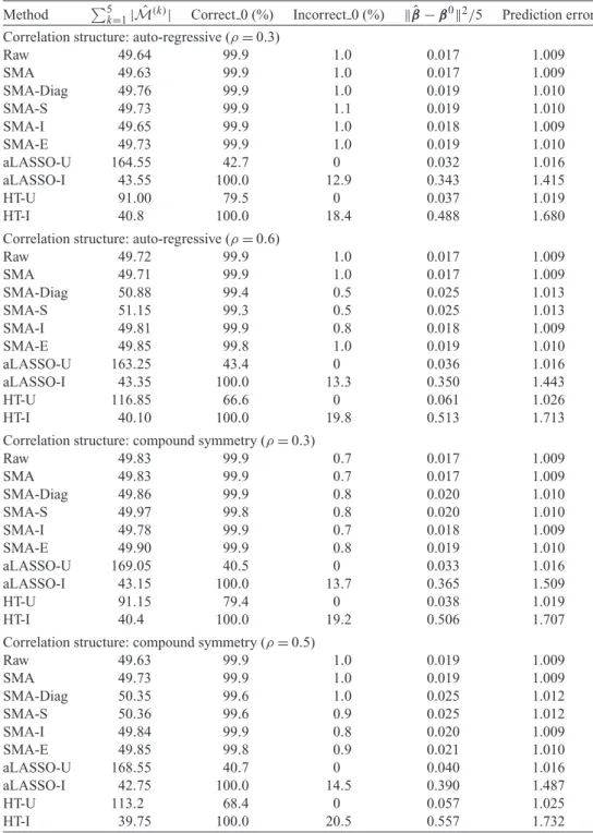
Table 1. Comparison of the SMA with other methods under the homogeneous structure for p=50
Method 5k=1| ˆM(k)| Correct 0 (%) Incorrect 0 (%) ˆβ−β02/5 Prediction error Correlation structure: auto-regressive (ρ=0.3)
Raw 49.64 99.9 1.0 0.017 1.009
SMA 49.63 99.9 1.0 0.017 1.009
SMA-Diag 49.76 99.9 1.0 0.019 1.010
SMA-S 49.73 99.9 1.1 0.019 1.010
SMA-I 49.65 99.9 1.0 0.018 1.009
SMA-E 49.73 99.9 1.0 0.019 1.010
aLASSO-U 164.55 42.7 0 0.032 1.016
aLASSO-I 43.55 100.0 12.9 0.343 1.415
HT-U 91.00 79.5 0 0.037 1.019
HT-I 40.8 100.0 18.4 0.488 1.680
Correlation structure: auto-regressive (ρ=0.6)
Raw 49.72 99.9 1.0 0.017 1.009
SMA 49.71 99.9 1.0 0.017 1.009
SMA-Diag 50.88 99.4 0.5 0.025 1.013
SMA-S 51.15 99.3 0.5 0.025 1.013
SMA-I 49.81 99.9 0.8 0.018 1.009
SMA-E 49.85 99.8 1.0 0.019 1.010
aLASSO-U 163.25 43.4 0 0.036 1.016
aLASSO-I 43.35 100.0 13.3 0.350 1.443
HT-U 116.85 66.6 0 0.061 1.026
HT-I 40.10 100.0 19.8 0.513 1.713
Correlation structure: compound symmetry (ρ=0.3)
Raw 49.83 99.9 0.7 0.017 1.009
SMA 49.83 99.9 0.7 0.017 1.009
SMA-Diag 49.86 99.9 0.8 0.020 1.010
SMA-S 49.97 99.8 0.8 0.020 1.010
SMA-I 49.78 99.9 0.7 0.018 1.009
SMA-E 49.90 99.9 0.8 0.019 1.010
aLASSO-U 169.05 40.5 0 0.033 1.016
aLASSO-I 43.15 100.0 13.7 0.365 1.509
HT-U 91.15 79.4 0 0.038 1.019
HT-I 40.4 100.0 19.2 0.506 1.707
Correlation structure: compound symmetry (ρ=0.5)
Raw 49.63 99.9 1.0 0.019 1.009
SMA 49.73 99.9 1.0 0.019 1.009
SMA-Diag 50.35 99.6 1.0 0.025 1.012
SMA-S 50.36 99.6 0.9 0.025 1.012
SMA-I 49.84 99.9 0.8 0.020 1.009
SMA-E 49.85 99.8 0.9 0.021 1.010
aLASSO-U 168.55 40.7 0 0.040 1.016
aLASSO-I 42.75 100.0 14.5 0.390 1.487
HT-U 113.2 68.4 0 0.057 1.025
estimation errors and prediction errors. The results for the heterogeneous structure show similar patterns (see Table S1a of supplementary material available atBiostatisticsonline). Indeed, under the heterogeneous structure, the aLASSO-I and HT-I are bound to fail by their design.
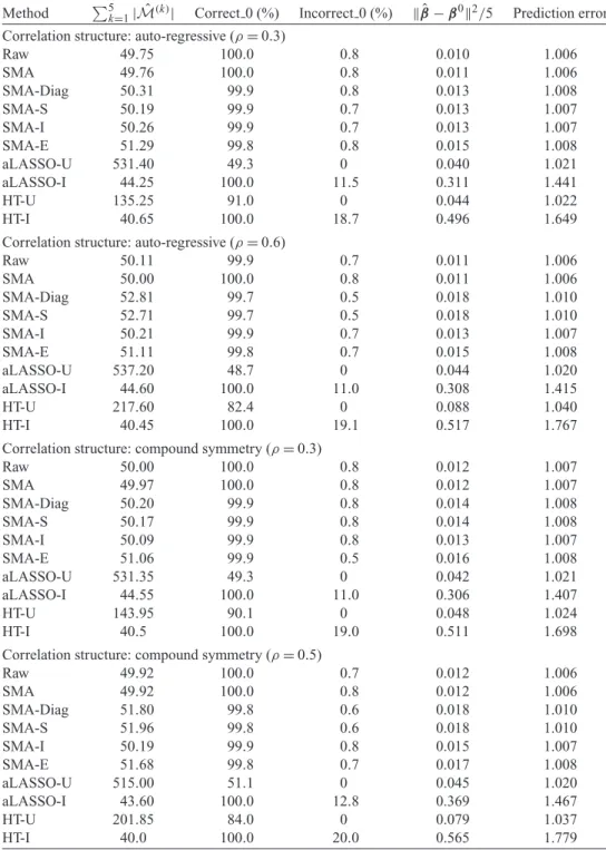
3.2 Large dimensions
We increased the number of SNPs to 200 and set the sample sizes to 2000, 1900, 1800, 1900, and 2000. For the SMA-E, we simulated an external panel of 1000 subjects. The results are shown in Table2and Table S1b of supplementary material available atBiostatisticsonline. The SMA method continues to perform similarly to the Raw method. In addition, the SMA is able to capture most of the important SNPs, while maintaining a model size that is close to the true model size. The SMA-Diag and SMA-S are less efficient than the SMA but still possess the desirable model sparsity. The SMA-I and SMA-E maintain their model sparsity with quite accurate estimation of parameters. In contrast, the aLASSO-U and HT-U include a large number of noise SNPs, while the aLASSO-I and HT-I tend to miss important SNPs.
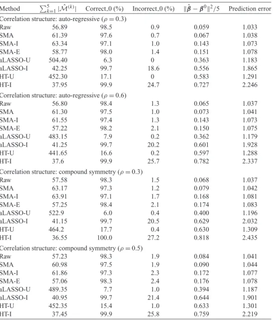
3.3 p>n
Whenpis greater thann, variable selection in meta-analysis becomes extremely challenging. Our SMA is based on summary statistics, but the ordinary least-squares (OLS) estimates cannot be obtained when p>n. Under such a situation, it is necessary to reduce the dimension from an ultra-high level to a level that is amenable to most variable selection methods. We propose to first conduct marginal screening to reduce the dimension to be smaller thann and then obtain the summary statistics based on the reduced set of variables. This strategy is in the same vein as the sure independence screening (SIS) ofFan and Lv(2008). Because the SIS theory ensures that all important variables are preserved after the marginal screening, the selection consistency of the SMA with marginal screening is guaranteed. We evaluated the empirical performance in simulation studies. To have a fair comparison, the aLASSO-U, aLASSO-I, HT-U, and HT-I were also conducted after the SIS procedure. We set the sample sizes of the five studies to 600, 500,
600, 500, and 400. The dimension p was set to 10 000. We first performed the marginal screening on
each study to reduce the dimension from pton/(3 log(n))and then took a union of the reduced sets of SNPs for subsequent variable selection. As shown in Table3, the SMA model still has a reasonable model size, with the parameter-estimation error and the prediction error comparable with the Raw method. The aLASSO-U, aLASSO-I, HT-U, and HT-I either lose model sparsity or miss important SNPs, thus resulting in higher estimation errors and prediction errors, as was the case in the previous simulation studies.
3.4 Other considerations
We also addressed several other issues on sparse meta-analysis, such as a model structure different from the homogeneous and heterogeneous structures, the influence of sparsity on variable selection, different sets of candidate variables among studies, and the influence of screening on variable selection. The interested readers are referred to Section B of supplementary material available atBiostatisticsonline.
4. REAL DATA ANALYSIS
Table 2.Comparison of the SMA with other methods under the homogeneous structure for p=200
Method 5k=1| ˆM(k)| Correct 0 (%) Incorrect 0 (%) ˆβ−β02/5 Prediction error Correlation structure: auto-regressive (ρ=0.3)
Raw 49.75 100.0 0.8 0.010 1.006
SMA 49.76 100.0 0.8 0.011 1.006
SMA-Diag 50.31 99.9 0.8 0.013 1.008
SMA-S 50.19 99.9 0.7 0.013 1.007
SMA-I 50.26 99.9 0.7 0.013 1.007
SMA-E 51.29 99.8 0.8 0.015 1.008
aLASSO-U 531.40 49.3 0 0.040 1.021
aLASSO-I 44.25 100.0 11.5 0.311 1.441
HT-U 135.25 91.0 0 0.044 1.022
HT-I 40.65 100.0 18.7 0.496 1.649
Correlation structure: auto-regressive (ρ=0.6)
Raw 50.11 99.9 0.7 0.011 1.006
SMA 50.00 100.0 0.8 0.011 1.006
SMA-Diag 52.81 99.7 0.5 0.018 1.010
SMA-S 52.71 99.7 0.5 0.018 1.010
SMA-I 50.21 99.9 0.7 0.013 1.007
SMA-E 51.11 99.8 0.7 0.015 1.008
aLASSO-U 537.20 48.7 0 0.044 1.020
aLASSO-I 44.60 100.0 11.0 0.308 1.415
HT-U 217.60 82.4 0 0.088 1.040
HT-I 40.45 100.0 19.1 0.517 1.767
Correlation structure: compound symmetry (ρ=0.3)
Raw 50.00 100.0 0.8 0.012 1.007
SMA 49.97 100.0 0.8 0.012 1.007
SMA-Diag 50.20 99.9 0.8 0.014 1.008
SMA-S 50.17 99.9 0.8 0.014 1.008
SMA-I 50.09 99.9 0.8 0.013 1.007
SMA-E 51.06 99.9 0.5 0.016 1.008
aLASSO-U 531.35 49.3 0 0.042 1.021
aLASSO-I 44.55 100.0 11.0 0.306 1.407
HT-U 143.95 90.1 0 0.048 1.024
HT-I 40.5 100.0 19.0 0.511 1.698
Correlation structure: compound symmetry (ρ=0.5)
Raw 49.92 100.0 0.7 0.012 1.006
SMA 49.92 100.0 0.8 0.012 1.006
SMA-Diag 51.80 99.8 0.6 0.018 1.010
SMA-S 51.96 99.8 0.6 0.018 1.010
SMA-I 50.19 99.9 0.8 0.015 1.007
SMA-E 51.68 99.8 0.7 0.017 1.008
aLASSO-U 515.00 51.1 0 0.045 1.020
aLASSO-I 43.60 100.0 12.8 0.369 1.467
HT-U 201.85 84.0 0 0.079 1.037
Table 3. Performance of the SMA and other methods with marginal screening under the homogeneous structure for p>n
Method 5k=1| ˆM(k)| Correct 0 (%) Incorrect 0 (%) ˆβ−β02/5 Prediction error Correlation structure: auto-regressive (ρ=0.3)
Raw 56.89 98.5 0.9 0.059 1.033
SMA 61.39 97.6 0.7 0.067 1.038
SMA-I 63.34 97.1 1.0 0.143 1.073
SMA-E 58.77 98.0 1.4 0.151 1.078
aLASSO-U 504.40 6.3 0 0.363 1.183
aLASSO-I 42.25 99.7 18.6 0.556 1.865
HT-U 452.30 17.1 0 0.583 1.291
HT-I 37.95 99.9 24.7 0.727 2.246
Correlation structure: auto-regressive (ρ=0.6)
Raw 56.80 98.4 1.3 0.065 1.037
SMA 61.30 97.5 1.0 0.073 1.041
SMA-I 61.55 97.4 1.3 0.143 1.073
SMA-E 57.22 98.2 2.1 0.150 1.075
aLASSO-U 483.15 7.9 0.2 0.362 1.179
aLASSO-I 41.25 99.7 20.2 0.601 1.928
HT-U 441.65 16.6 0.2 0.597 1.288
HT-I 37.6 99.9 25.7 0.782 2.337
Correlation structure: compound symmetry (ρ=0.3)
Raw 57.58 98.3 1.5 0.068 1.037
SMA 63.17 97.3 1.2 0.079 1.042
SMA-I 63.91 97.1 1.7 0.168 1.081
SMA-E 57.25 98.4 2.1 0.174 1.083
aLASSO-U 522.9 6.0 0.4 0.400 1.196
aLASSO-I 41.15 99.7 20.5 0.629 2.032
HT-U 464.2 17.7 0.4 0.630 1.309
HT-I 36.55 100.0 27.2 0.818 2.435
Correlation structure: compound symmetry (ρ=0.5)
Raw 57.23 98.3 1.9 0.084 1.041
SMA 60.98 97.5 1.9 0.090 1.044
SMA-I 61.86 97.3 2.3 0.172 1.077
SMA-E 57.06 98.3 2.4 0.176 1.078
aLASSO-U 489.35 7.7 1.0 0.394 1.187
aLASSO-I 40.95 99.7 21.4 0.644 1.901
HT-U 452.35 15.4 1.0 0.633 1.301
HT-I 37.45 99.9 25.8 0.759 2.219
Note:p=10 000 and the sample sizes range from 400 to 600. The Correct 0 (%) and Incorrect 0 (%) were based on the dimensions after the SIS procedure. The SMA-E used an external panel of 1000 subjects.
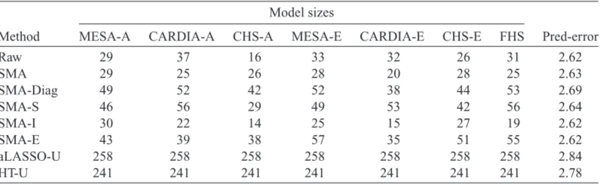
Table 4.Variable selection in seven studies (i.e., FHS, MESA-A, MESA-E, CARDIA-A, CARDIA-E, CHS-A, and CHS-E) followed by prediction in the ARIC-A and ARIC-E studies
Model sizes
Method MESA-A CARDIA-A CHS-A MESA-E CARDIA-E CHS-E FHS Pred-error
Raw 29 37 16 33 32 26 31 2.62
SMA 29 25 26 28 20 28 25 2.63
SMA-Diag 49 52 42 52 38 44 53 2.69
SMA-S 46 56 29 49 53 42 56 2.64
SMA-I 30 22 14 25 15 27 19 2.62
SMA-E 43 39 38 57 35 51 55 2.62
aLASSO-U 258 258 258 258 258 258 258 2.84
HT-U 241 241 241 241 241 241 241 2.78
lipidpc1, which is a continuous variable derived from the principal component analysis of several fasting serum measurements: low-density lipoprotein, high-density lipoprotein, triglycerides, apolipoprotein A1, and apolipoprotein B;lipidpc1was found to be associated with genetic loci implicated in obesity, athero-geneic dyslipidemia, and glucose metabolism (Averyand others,2011). We conducted marginal screening (details in Section C of supplementary material available atBiostatisticsonline) which yielded 276 can-didate SNPs for variable selection. The number of SNPs studied herein is in accordance with the SIS theory, as well as practical variable selection in GWAS (Wuand others,2009). We adjusted the values of lipidpc1by environmental covariates (i.e., age, gender, and study site), as well as the first 10 eigenvec-tors from the principal component analysis of the GWAS SNPs to account for the population substructure (Averyand others,2011). We then applied the SMA and other methods to the adjustedlipidpc1and the 276 SNPs.
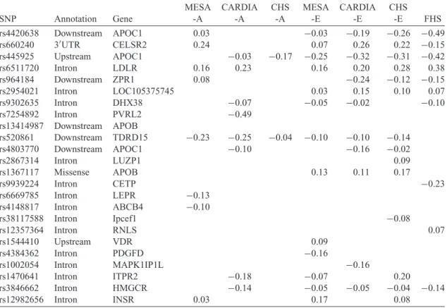
Table 5.Estimated regression coefficients for some selected SNPs in the SMA model
MESA CARDIA CHS MESA CARDIA CHS
SNP Annotation Gene -A -A -A -E -E -E FHS
rs4420638 Downstream APOC1 0.03 −0.03 −0.19 −0.26 −0.49
rs660240 3UTR CELSR2 0.24 0.07 0.26 0.22 −0.15
rs445925 Upstream APOC1 −0.03 −0.17 −0.25 −0.32 −0.31 −0.42
rs6511720 Intron LDLR 0.16 0.23 0.16 0.20 0.28 0.38
rs964184 Downstream ZPR1 0.08 −0.24 −0.12 −0.15
rs2954021 Intron LOC105375745 0.03 0.15 0.10 0.07
rs9302635 Intron DHX38 −0.07 −0.05 −0.02 −0.10
rs7254892 Intron PVRL2 −0.49
rs13414987 Downstream APOB
rs520861 Downstream TDRD15 −0.23 −0.25 −0.04 −0.10 −0.10 −0.14
rs4803770 Downstream APOC1 −0.10 −0.16 −0.02
rs2867314 Intron LUZP1 0.09
rs1367117 Missense APOB 0.13 0.11 0.17
rs9939224 Intron CETP −0.23
rs6669785 Intron LEPR −0.13
rs4148817 Intron ABCB4 −0.10
rs38117588 Intron Ipcef1 −0.08
rs12357364 Intron RNLS 0.07
rs1544410 Upstream VDR 0.09
rs4384362 Intron PDGFD −0.16
rs1002054 Intron MAPK1IP1L −0.16
rs1470641 Intron ITPR2 −0.18 −0.07 0.20
rs3846662 Intron HMGCR −0.14 −0.05 −0.05 −0.04 −0.14
rs12982656 Intron INSR 0.03 0.17 0.08
Note: Zero estimates are left blank. Annotation is based on dbSNP (http://www.ncbi.nlm.nih.gov/snp).
population is more homogeneous than the latter. The meta-analysis of multiple studies also captures SNPs that are (partly) missed by the individual aLASSO. For example, we observe that rs4420638 is captured in five studies by the SMA, but only in three studies by the individual aLASSO; likewise, rs6511720 is captured in seven studies by the SMA-Diag, but only in six studies by the individual aLASSO.
To investigate the prediction performance, we tested the SNPs selected by the eight methods on the ARIC-A and ARIC-E. We chose the active SNPs from the CARDIA-A and CARDIA-E for prediction, as these two studies are clinically similar to the ARIC studies and have well-balanced sample sizes for the two race groups. We assessed the prediction accuracy by randomly dividing each of the ARIC-A and ARIC-E into two halves, using one half to estimate the regression coefficients (via unpenalized linear regression) and the other half to calculate the prediction error. As shown in Table4, the SMA, the SMA-Diag, and other SMA-derived methods achieve higher prediction accuracies than the aLASSO-U and HT-U. The larger prediction errors of the aLASSO-U and HT-U methods are likely due to their large model sizes, demonstrating the importance of variable selection when predicting genetic risks.
5. DISCUSSION
meta-analysis. The proposed methods are particularly useful for prospectively planned meta-analysis, in which the participating studies coordinate with each other to report appropriate summary statistics. We anticipate that our approach will find its applications in the forthcoming era of big data where it is imprac-tical to collect or store all of the raw data.
Our theoretical and numerical studies demonstrate that summary statistics can replace raw data for variable selection in meta-analysis, at least in the asymptotic sense, when full covariance matrices are available. In a similar spirit (although not in the context of variable selection),Lin and Zeng(2010) showed that summary statistics are asymptotically equivalent to raw data for meta-analysis under the fixed-effects model. We conjecture that if the first part of equation (2.1) is replaced by other suitable risk functions, then the asymptotic equivalence between summary statistics and raw data will continue to hold. If the penalty term in equation (2.1) is replaced by other reasonable penalties, such as group LASSO and group SCAD, then the asymptotic equivalence is also expected to hold. Which risk function or penalty term to use should depend on the scientific nature of the problem and the modeling aims of the investigators.
Although the penalty term in (2.1) is similar to that ofZhou and Zhu(2010), our paper deals with a very different problem.Zhou and Zhu(2010) considered group selection for a single dataset, with each group consisting of different variables (e.g., multiple genes in one pathway). In our case, each group corresponds to the same variable in multiple studies. The work ofZhou and Zhu(2010) requires access to raw data. In contrast, our approach is based solely on summary statistics and can even accommodate situations where the covariance information is not available. Because we address a different problem and work with (poten-tially incomplete) summary statistics instead of raw data, our technical arguments and theoretical results are somewhat different from those ofZhou and Zhu(2010). We have established the oracle property of the SMA and the selection consistency and estimation consistency for arbitrary working covariance matrices. We have implicitly assumed thatβ˜kis obtained under a multi-variable model. Published studies, how-ever, may report regression coefficients that are estimated with one covariate in the model at a time. If the covariates are approximately uncorrelated, then the regression coefficients from the multi-variable and single-variable models are similar. When the covariance matrix of the covariates is available from one of the participating studies or from an external panel, such as the Hapmap and 1000 Genomes, we can recover the regression coefficients in the multi-variable model by adjusting the regression coefficients estimated from the single-variable models through simple matrix multiplication.
It would be worthwhile to enhance the capability of the SMA to tackle the “p>n” situation. In this article, we adopt the SIS theory to reduce the dimension to a manageable size and then apply the SMA for variable selection. This strategy is practically useful and seems to work well. An alternative approach would be to directly handle the “p>n” challenge, without implementing any pre-screening procedure. However, such methods are still very limited, and their applications to large datasets (such as those derived from GWAS) may be severely hindered by the excessively large number of variables. Indeed, it is still unclear what kind of summary statistics one can/should collect for data with “p>n.”
Recently, Guan and Stephens (2011) proposed a Bayesian variable selection approach, which was
shown to be capable of detecting weak effects in GWAS. In addition,Pickrell(2014) proposed a Bayesian hierarchical model for integrating functional genomic information with GWAS data. It would be worth-while to extend such Bayesian methods to the setting of variable selection in meta-analysis and make a comparison with the frequentist methods presented in this paper.
SUPPLEMENTARY MATERIAL
Supplementary material is available athttp://biostatistics.oxfordjournals.org.
ACKNOWLEDGMENTS
The authors are grateful to Shuangge Ma, Yufeng Liu, and Donglin Zeng for discussions and to Qing Duan and Yun Li for assistance with the 1000 Genomes data. They also thank an associate editor and two referees for constructive comments.Conflict of Interest: None declared.
FUNDING
This work was supported by National Institutes of Health grants (R01 CA082659, P01 CA142538, and R37GM047845) and National Science Foundation grants (DBI-1261830 and DMS-1418172).
REFERENCES
AVERY, C.,HE, Q.,NORTH, K.,AMBITE, J.,BOERWINKLE, E.,FORNAGE, M.,HINDORFF, L.,KOOPERBERG, C.,MEIGS, J.,PANKOW, J.and others(2011). A phenomics-based strategy identifies loci on APOC1, BRAP, and PLCG1 associated with metabolic syndrome phenotype domains.PLoS Genetics7(10), e1002322.
CHEN, H.,MANNING, A. K.ANDDUPUIS, J. (2012). A method of moments estimator for random effect multivariate meta-analysis.Biometrics68(4), 1278–1284.
CHEN, Q. ANDWANG, S. (2013). Variable selection for multiply-imputed data with application to dioxin exposure study.Statistics in Medicine32(21), 3646–3659.
DERSIMONIAN, R.ANDLAIRD, N. (1986). Meta-analysis in clinical trials.Controlled Clinical Trials7(0), 177–88. FAN, J.ANDLV, J. (2008). Sure independence screening for ultrahigh dimensional feature space.Journal of the Royal
Statistical Society: Series B70(5), 849–911.
FRIEDMAN, R.,HASTIE, T.,H¨OFLING, H.ANDTIBSHIRANI, R. (2007). Pathwise coordinate optimization.The Annals of Applied Statistics1(2), 302–332.
Global Lipids Genetics Consortium (2013). Discovery and refinement of loci associated with lipid levels.Nature Genetics45(11), 1274–1283.
GUAN, Y.ANDSTEPHENS, M. (2011). Bayesian variable selection regression for genome-wide association studies and other large-scale problems.The Annals of Applied Statistics5(3), 1780–1815.
HU, Y. J.,BERNDT, S. I., GUSTAFSSON, S., GANNA, A., GENETIC INVESTIGATION OF ANTHROPOMETRIC TRAITS (GIANT) CONSORTIUM,HIRSCHHORN, J.,NORTH, K. E.,INGELSSON, E. andLIN, D. Y. (2013) Meta-analysis of gene-level associations for rare variants based on single-variant statistics.The American Journal of Human Genet-ics9(2), 236–248.
JACKSON, D.,WHITE, I. R.ANDTHOMPSON, S. G. (2010). Extending DerSimonian and Laird’s methodology to perform multivariate random effects meta-analyses.Statistics in Medicine29(12), 1282–1297.
LANGO, H. A.,ESTRADA, K.,LETTRE, G.,BERNDT, S. I.,WEEDON, M. N.,RIVADENEIRA, F.,WILLER, C. J.,JACKSON, A. U.,VEDANTAM, S.,RAYCHAUDHURI, S.and others(2010). Hundreds of variants clustered in genomic loci and biological pathways affect human height.Nature467(7317), 832–838.
LIU, D.,PELOSO, G.,ZHAN, X.,HOLMEN, O.,ZAWISTOWSKI, M.,FENG, S.,NIKPAY, M.,AUER, P.,GOEL, A.,ZHANG, He.and others(2014). Meta-analysis of gene-level tests for rare variant association.Nature Genetics46(2), 200– 204.
LIU, F.,DUNSON, D. ANDZOU, F. (2011). High-dimensional variable selection in meta-analysis for censored data. Biometrics67(2), 504–512.
MA, S.,HUANG, J.ANDSONG, X. (2011). Integrative analysis and variable selection with multiple high-dimensional data sets.Biostatistics12(4), 763–75.
NOBLE, J. (2006). Meta-analysis: methods, strengths, weaknesses, and political uses. Journal of Laboratory and Clinical Medicine147(1), 7–20.
PICKRELL, J. (2014). Joint analysis of functional genomic data and genome-wide association studies of 18 human traits.American Journal of Human Genetics94(4), 559–73.
TENENHAUS, A.,PHILIPPE, C.,GUILLEMOT, V.,CAO, K. A.,GRILL, J. andFROUIN, V. (2014). Variable selection for generalized canonical correlation analysis.Biostatistics15(3), 569–83.
TIBSHIRANI, R. (1996). Regression shrinkage and selection via the Lasso.Journal of the Royal Statistical Society: Series B58(1), 267–288.
WANG, H. (2009). Forward regression for ultra-high dimensional variable screening.Journal of the American Statis-tical Association104(488), 1512–1524.
WANG, H.ANDLENG, C. (2007). Unified LASSO estimation by least squares approximation.Journal of the American Statistical Association102(479), 1039–1048.
WU, T. T.,CHEN, Y. F.,HASTIE, T.,SOBEL, E.ANDLANGE, K. (2009). Genome-wide association analysis by lasso penalized logistic regression.Bioinformatics25(6), 714–721.
ZEISEL, S. (2007). Nutrigenomics and metabolomics will change clinical nutrition and public health practice: insights from studies on dietary requirements for choline.The American Journal of Clinical Nutrition86(3), 542–548. ZHOU, N.ANDZHU, J. (2010). Group variable selection via a hierarchical lasso and its oracle property.Statistics and
Its Interface3(4), 557–574.
ZOU, H. (2006). The adaptive LASSO and its oracle properties.Journal of the American Statistical Association 101(476), 1418–1429.