CHARACTERIZING HYPERPOLARIZED 129Xe DEPOLARIZATION MECHANISMS DURING CONTINUOUS-FLOW SPIN EXCHANGE OPTICAL PUMPING AND AS A
SOURCE OF IMAGE CONTRAST
Alex Burant
A dissertation submitted to the faculty at the University of North Carolina at Chapel Hill in partial fulfillment of the requirements for the degree of Doctor of Philosophy in the
Department of Physics and Astronomy.
Chapel Hill 2018
Approved by:
Rosa Tamara Branca Thomas Clegg
c O2018 Alex Burant
ABSTRACT
Alex Burant: CHARACTERIZING HYPERPOLARIZED 129Xe
DEPOLARIZATION MECHANISMS DURING CONTINUOUS-FLOW SPIN EXCHANGE OPTICAL PUMPING AND AS A SOURCE OF IMAGE
CONTRAST.
(Under the direction of Rosa Tamara Branca.)
Xenon-129 has become the isotope of choice for applications of hyperpolarized (HP) noble gases in magnetic resonance imaging (MRI) and spectroscopy due to its lower cost and higher availability compared to 3He, relatively high tissue solubility, and wide range of chemical shifts. As the signal achieved in HP gas MRI is directly related to the nuclear spin polarization, the production of large volumes of highly polarized 129Xe is paramount.
While near unity levels of xenon polarization have been achieved in optical cells using stopped-flow spin exchange optical pumping (SEOP), continuous-flow SEOP is the most widely used method for clinical applications as it enables the production of large volumes of hyperpolarized gas, which are necessary for imaging applications in humans. However, polarization levels achieved via continuous-flow SEOP are well below the theoretically pre-dicted values. In this dissertation,129Xe relaxation mechanisms that are often ignored during continuous-flow SEOP are investigated, through both simulations and experiments, to quan-tify their effects.
Then, the effect of diffusion-mediated depolarization of 129Xe gas in magnetic field in-homogeneities during continuous-flow SEOP is determined. The results indicate that xenon diffusion in regions in which the magnetic field abruptly changes strength and direction can be a major source of depolarization during continuous-flow SEOP. As such, care should be taken in the design of the SEOP setup to avoid these gradients in the flow path of the HP gas. In the absence of such large magnetic field gradients, wall collisions remain the major contributing factor to gas-phase spin relaxation.
Depolarization in magnetic field gradients can also be a source of image contrast for magnetic resonance imaging. To this end, the effects of longitudinal and transverse spin relaxation are separated and characterized for hyperpolarized 129Xe diffusing near SPIONs using finite element analysis and Monte Carlo simulations. Simulations demonstrate that signal loss near SPIONs is dominated by transverse relaxation, with little contribution from longitudinal relaxation. In addition, experimental and computational work clearly show that the high diffusion coefficient of xenon does not provide appreciable sensitivity enhancement to SPIONs at the length scales typically probed by MRI.
ACKNOWLEDGMENTS
Getting here, six years later, was possible thanks to an unknowable number of people. First and foremost, I am thankful for the guidance and support of my advisor, Tamara Branca. I appreciate you taking a chance on me after my first year and allowing me to find my feet as a scientist. You are the definition of hard work (I still don’t know how you do it) and a model mentor, researcher, and educator.
I am thankful to the entire Branca group including Le Zhang, Drew McCallister, and Michael Antonacci. You have provided support, assistance, and helpful conversations to not only complete but understand all the work presented here. I would not want to run scans at 6 AM or on the weekend with anyone else.
I am thankful to my other committee members, Tom Clegg, Reyco Henning, Laurie McNeil, and Jack Ng, for their patience, flexibility, willingness to serve, and fortitude to read this dissertation.
Thank you to Duane Deardorff, Alice Churukian, Jennifer Weinberg-Wolf, and Stefan Jeglinski for the opportunity to learn from and teach with you. I appreciate all that you have done to make me a better instructor and prepare me to be a physics educator.
This journey would not have been possible without the support and encouragement of my family and friends. My friends have been there the entire way to celebrate and commiserate all that goes into being a graduate student. My family has been a constant source of support, not just during my time at UNC, but throughout my life. I would especially like to thank my parents. I cannot say or do enough to thank you for all that you have done for me.
TABLE OF CONTENTS
LIST OF FIGURES . . . x
LIST OF TABLES . . . xi
LIST OF ABBREVIATIONS AND SYMBOLS . . . xii
1 INTRODUCTION . . . 1
1.1 Spin Exchange Optical Pumping of Noble Gas Nuclei . . . 5
1.2 Theoretical Model of Noble Gas Polarization . . . 12
1.3 Depolarization Mechanisms of Hyperpolarized Gases . . . 16
1.4 Overview of Contents . . . 20
2 CHARACTERIZATION OF FLUID FLOW IN CONTINUOUS-FLOW SPIN EXCHANGE OPTICAL PUMPING CELLS . . . 22
2.1 The Discrepancy between Theoretical and Experimental Nuclear Spin Polarization of 129Xe . . . . 22
2.2 Optical Cell Designs . . . 24
2.3 Computational Fluid Dynamics Simulations of Flow within the Op-tical Cell . . . 25
2.3.1 Plug Flow and Fully Developed Flow at the Cell Inlet . . . 26
2.3.2 Effects of Convection on the Flow Field within the Optical Cell . . . 33
2.3.3 Modeling Rubidium Vaporization within the Presaturation Region . . 35
2.4 Conclusions . . . 39
3.1 Effect of Magnetic Field Gradients on129Xe Depolarization . . . 42
3.2 Theoretical Background . . . 44
3.3 Simulating Depolarization of129Xe Gas in Magnetic Field Gradients . . . . . 45
3.3.1 Magnet Designs and Models . . . 46
3.3.2 Determination of the Magnetic Field Distribution . . . 47
3.3.3 Theoretical T1 of HP 129Xe Gas in the Cold Finger After Thawing . 50 3.4 Experimental Determination of T1 in the Cold Finger . . . 52
3.5 Conclusions . . . 55
4 HP 129Xe RELAXATION IN MAGNETIC FIELD GRADIENTS GENERATED BY SUPERPARAMAGNETIC IRON OXIDE NANOPAR-TICLES . . . 57
4.1 Introduction . . . 57
4.2 Transverse and Longitudinal Relaxation in Magnetic Field Gradients . . . . 59
4.2.1 Transverse Magnetization Decay in Uniform Magnetic Field Gradients 59 4.2.2 The In-between case of the Linear Gradient Approximation . . . 62
4.2.3 Approximation Regimes for Transverse Relaxation in Non-uniform Magnetic Field Gradients . . . 63
4.2.4 Longitudinal Relaxation in Magnetic Field Inhomogeneities . . . 65
4.3 Simulated HP129Xe Image Contrast . . . 65
4.3.1 Test of Finite Element Analysis Accuracy for Model Systems . . . 66
4.3.2 Longitudinal and Transverse Relaxation During Restricted Dif-fusion in a Cubic Geometry . . . 69
4.3.3 Generating Simulated MR Images in a Conical Phantom . . . 71
4.3.4 Simulated Magnetic Resonance Images of a Mouse Lung Model . . . 72
4.4 Experimental Validation of 129Xe Image Contrast near SPIONs . . . . 73
4.4.3 Experimental Imaging of Conical Centrifuge Tube . . . 75
4.4.4 In vivo MRI of Mouse Lungs in the Presence of SPIONs . . . 76
4.5 Results and Discussion . . . 77
4.6 Conclusions . . . 87
5 CONCLUSIONS & OUTLOOK . . . 89
5.1 Fluid Flow in Continuous-flow Optical Cells . . . 89
5.2 Depolarization in Magnetic Field Gradients . . . 90
5.3 Future Outlook . . . 91
LIST OF FIGURES
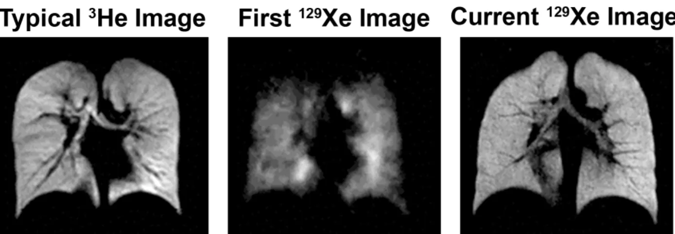
1.1 Comparison of HP 3He and 129Xe Lung Ventilation Images in Healthy Adults . 3
1.2 SEOP System Schematic . . . 7
1.3 Diagram of Depopulation Optical Pumping of Rubidium . . . 8
1.4 Spin Exchange Mechanisms for Rubidium and Xenon . . . 9
1.5 Polarean 9800 129Xe Hyperpolarizer and Continuous-flow SEOP Schematic . . . 11
2.1 CAD Models of Optical Cell Designs . . . 25
2.2 Developing Flow in a Circular Pipe . . . 27
2.3 CAD Models of Plug Flow Optical Cells . . . 29
2.4 Plug Flow and Fully Developed Flow Velocity Profiles . . . 30
2.5 Plug Flow and Fully Developed Flow Results . . . 31
2.6 Histogram Plots of Residency Time Within Optical Cells . . . 32
2.7 Effect of Gravitational Force on Fluid Flow with Heat Transfer . . . 34
2.8 CAD Models of Optical Cell Designs with Rubidium . . . 36
2.9 Effect of Rubidium Vaporization on Flow Field in Rear Inlet Cell . . . 37
2.10 Histogram Plots of Residency Time Within Optical Cells with Heat Transfer . . 38
3.1 Magnetic-decoupling Factor as a Function of Field Strength . . . 45
3.2 CAD model of Continuous-flow SEOP Setup . . . 46
3.3 3D View of Both Permanent Magnet Designs . . . 47
3.4 Field Maps of Both Permanent Magnet Designs . . . 49
3.5 Arc of Low Magnetic Field Strength in Original Magnet Design . . . 50
3.6 Close up of Magnetic Field Strength in Original Magnet Design . . . 51
3.7 Experimental T1 Relaxation Curves for Each Permanent Magnet Design . . . . 54
4.2 Comparison of Analytical and Numerical Results for Infinite Cylinder in
Applied Magnetic Field . . . 68 4.3 Cubic Geometry to Test Restricted Diffusion of Xenon Gas . . . 69 4.4 Comparison of Frequency Offset for Simulated and Experimental MR Images . . 75 4.5 Effect of Boundary on Contrast Generated by HP 129Xe Near SPIONs . . . . . 79 4.6 Relative Contribution of T1 and T2? to Relaxation of 129Xe near SPIONs . . . . 80 4.7 Effect of Structural Length on Image Contrast of129Xe During Restricted
Diffusion Around SPIONs . . . 81 4.8 Effect of Echo Time on Image Contrast of129Xe at Various Length Scales
Near SPIONs . . . 82 4.9 Simulated Xenon Magnetization Decay Near and Far from SPIONs . . . 83 4.10 Comparison of Experimental and Simulated 129Xe Image Contrast near SPIONs 84 4.11 Simulated Xenon Magnetization Decay Near SPIONs in Conical
LIST OF TABLES
1.1 Spin Destruction Cross Sections for Rb Binary Collisions . . . 13 1.2 Measured Coefficients for the Breakup of van der Waals Molecules by
Xenon and Nitrogen . . . 18 3.1 Atomic Diffusion Volumes . . . 52 4.1 Internal and External Field Changes for Simple Geometries, Including
LIST OF ABBREVIATIONS AND SYMBOLS
BC Binary Collisions
HP Hyperpolarized
HPXe Hyperpolarized Xenon
MRI Magnetic Resonance Imaging NMR Nuclear Magnetic Resonance SEOP Spin Exchange Optical Pumping SNR Signal-to-Noise Ratio
SPIONs SuperParamagnetic Iron Oxide Nanoparticles vdW van der Waals molecules
1H Hydrogen
3He Helium-3
CHAPTER 1: INTRODUCTION
The first demonstration of hyperpolarized (HP) gas magnetic resonance imaging (MRI) in a biological system occurred in 1994 when Albert et al. (1994) produced mouse lung images using hyperpolarized129Xe. Shortly thereafter, the firstin vivo images using hyperpolarized 3He were produced and work in hyperpolarized noble gas MRI took off. Hyperpolarized noble gas MRI offered a new frontier of imaging in the lungs that had previously been limited because of the low spin density of 1H in the void space of the lungs along with a variety of other confounding factors that make proton MRI in the lungs difficult (Wild et al., 2012).
There were many hurdles to overcome in the pursuit of using hyperpolarized noble gases to perform ventilation studies in the lungs. First,1H, the most often used nucleus in magnetic resonance, has the highest gyromagnetic ratio of all stable nuclei, which means using any other nucleus will immediately impart a penalty on the achievable signal. Second, noble gas density is three orders of magnitude lower than the density of 1H in the lungs even in the best case scenario of inhaling an entire inspiratory capacity (∼3.5 L) of noble gas. Even if inhaling that much noble gas were feasible, it is not allowed under current imaging protocols. To see how it is possible to overcome these obstacles, it is important to understand how signal is generated in MRI. The nuclear magnetic resonance (NMR) signal is proportional to:
Signal∝N ×µ×Ω0×P, (1.0.1)
γ, and the applied magnetic field strength, B0 (Ω0 = γB0). The magnetic moment is an intrinsic property of the atoms. Therefore, these are properties which cannot be changed. In the case of noble gases the spin density may also not be increased as there is a finite amount of gas that a subject can inhale. This leaves increasing the spin polarization as the only option to increase the signal generated by the noble gases. Hyperpolarization techniques are able to increase the nuclear spin polarization of noble gas nuclei by up to five orders of magnitude compared to their thermal equilibrium levels and provides the signal-to-noise ratio (SNR) necessary to produce void space images in the lungs.
Early work in hyperpolarized noble gas MRI centered around the use of hyperpolarized 3He. Hyperpolarized 3He MRI produced high SNR images in the lung to help better un-derstand lung function and structure and was able to provide anatomical information on ventilation defects caused by asthma, cystic fibrosis, and Chronic Obstructive Pulmonary Disease (COPD) (de Lange et al., 2006; Woodhouse et al., 2009; Evans et al., 2007). The decision to use3He was an easy one as hyperpolarized3He had been used for many years as a target in fundamental nuclear physics experiments including neutron detection and parity violation in the weak interaction between the proton and neutron (Johnson et al., 1995; Anthony et al., 1993; Coulter et al., 1988). This meant that the methods to polarize helium were understood and the polarization technology was well developed. The achievable polar-ization levels of helium were already greater than 50%, much higher than the polarpolar-izations achieved by 129Xe (Chen et al., 2014).
for everyone else to rise above $2000 per liter. Fortunately, 129Xe provides a cheap (∼$20 per liter for natural abundance) and effective alternative to 3He and can now reach similar polarization levels for comparable volumes of gas (Nikolaou et al., 2013).
For comparison, Figure 1.1 shows typical ventilation images that are possible today using both3He and 129Xe along with the first 129Xe human lung image produced by Mugler et al. (1997). As can be seen, the ventilation images achieved using hyperpolarized129Xe rival the SNR and resolution of those using hyperpolarized 3He. Along with providing high quality ventilation images of the lungs, 129Xe has other characteristics which make it appealing for use in in vivo MRI including its relatively high tissue solubility and wide range of chemical shifts. These properties, along with the higher nuclear spin polarization achieved in recent years, have enabled application of hyperpolarized 129Xe outside the lungs. HP 129Xe is now used as a probe for gas exchange in the lungs (Wang et al., 2017), for brain perfusion studies (Venkatesh et al., 2001; Rao et al., 2016), for the detection of highly perfused fatty tissues like brown adipose tissue (Branca et al., 2014), as well as a non-invasive temperature probe (Zhang et al., 2017).
In order to perform these experiments, liter volumes of highly polarized xenon gas are necessary. Since the signal-to-noise ratio is directly related to the polarization level of the gas (Equation 1.0.1), attaining the highest possible polarization is crucial. While there are multiple methods to hyperpolarize 129Xe, the most commonly used is spin exchange optical pumping (SEOP) performed in either batch-mode or continuous-flow (Barskiy et al., 2017). Though batch-mode hyperpolarization has seen polarization levels approaching unity
in situ, the maximum achievable polarizations for xenon occur at low xenon partial pressures (Nikolaou et al., 2013, 2014; Fink et al., 2005). This suggests that continuous-flow SEOP, which operates at much lower xenon partial pressures compared to batch-mode, should provide the means for obtaining the highest final xenon polarizations. However, continuous-flow hyperpolarizers have historically performed below predicted theoretical levels (Driehuys et al., 1996; Zook et al., 2002; Hersman et al., 2008).
Identifying the cause for the discrepancy between theoretical and experimental 129Xe polarization levels during continuous-flow SEOP remains one of the last obstacles faced by the field of HP gas MRI. This work focuses on possible mechanisms for polarization loss dur-ing continuous-flow SEOP which are either ignored or have been neglected to characterize their effects on the relaxation of HP 129Xe. In additions, the longitudinal and transverse relaxations of xenon near superparamagnetic iron oxide nanoparticles (SPIONs) are charac-terized.
1.1 Spin Exchange Optical Pumping of Noble Gas Nuclei
The idea of optically pumping alkali metal atoms to polarize electron spins was first shown in the Nobel Prize winning experiments performed by Kastler (1967). Kastler (1967) also theorized the possibility of transferring spin polarization from the electrons of alkali atoms to nuclei of noble gas atoms. The first experimental demonstrations of this technique were reported by Bouchiat et al. (1960) in 3He and by Grover (1978) in 129Xe who showed it could be accomplished in 129Xe at a much higher rate.
There are two possible methods for polarizing noble gas nuclei via exchange processes after optical pumping. The first, which is possible exclusively for 3He, is known as metasta-bility exchange optical pumping (MEOP) (Batz et al., 2011). This method takes advantage of a metastable state in 3He, which acts as a ground state during the optical pumping pro-cess, that can be populated by electron collisions within a plasma. Coupling between the nucleus and electrons in these atoms causes the optically-pumped orientation of the elec-trons to affect the nuclear spin orientation simultaneously. Finally, through metastability exchange collisions these atoms transfer their angular momentum to the 3He atoms which have remained in the true ground state to polarize the spins.
The second method is Spin Exchange Optical Pumping (SEOP), which is possible in a variety of nuclear spins including 3He and 129Xe. As the work presented here is achieved exclusively using 129Xe which is hyperpolarized via SEOP, this section will center on an explanation of this process and the hardware used in our lab to polarize the gas.
However, before the process of spin exchange optical pumping is described, a clear defini-tion of what it means for a noble gas to be “hyperpolarized” must be provided. As discussed previously,129Xe is a spin-1
the ground state and excited state to the total number of spins:
P = N+−N−
N++N−
. (1.1.1)
It is important to note that while this semiclassical definition is true for spin-12 systems, it breaks down for spins with spin quantum numbers greater thanI = 12, such as131Xe (I = 32). As this work will not be dealing with spins that exhibit spin quantum numbers greater than
I = 12, our semiclassical definition will suffice.
Spin Exchange Optical Pumping is a two-step process whereby angular momentum is transferred from the electronic spin of an alkali metal atom to the nuclear spin of a noble gas atom. In order for this exchange to occur, first the alkali metal vapor must be polar-ized through depopulation optical pumping and then angular momentum transfer can occur through spin exchange binary collisions or the formation of van der Waals molecules (Happer, 1972; Becker et al., 1994; Ruset et al., 2006; Schrank et al., 2009).
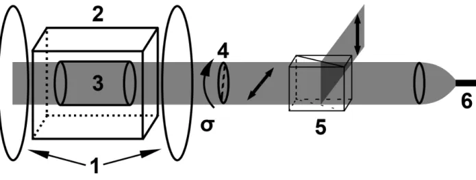
to between 100-200°C to produce an optically thick rubidium vapor while the Helmholtz coil produces a low, uniform magnetic field which causes Zeeman splitting of the alkali metals energy levels.
Figure 1.2: Example SEOP system schematic. 1. Helmholtz coil pair generating the polar-izing magnetic field. 2. Temperature controlled oven 3. Optical pumping cell containing an alkali metal vapor and the noble gas. 4. Quarter-wave plate to circularly polarize light. 5. Polarizing beamsplitter to separate horizontally and vertically polarized light. 6. Laser tuned to D1 transition of alkali metal.
The alkali metal vapor is continuously irradiated by the laser which is tuned to the D1 transition of the alkali metal. This causes the electrons in the ground state (5S1
2 for
rubidium) to transition into the excited state (5P1
2 for rubidium), but in order for optical
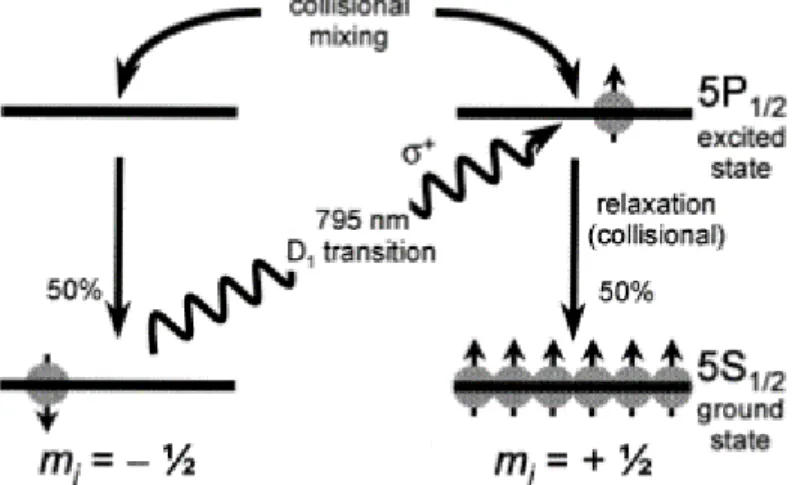
excited sublevels which means they relax to either of the ground state sublevels. Fortunately, since only one of the two ground states can absorb the angular momentum from the circularly polarized photons, the spins in other ground state become transparent to light. As a result, the “transparent” ground state becomes overpopulated and the electronic spins of the alkali atoms are said to be polarized. The depopulation of a single, alkali metal ground state sublevel is why this process is known as depopulation optical pumping.
Figure 1.3: Diagram showing the depopulation optical pumping of rubidium by laser light tuned to the 795 nm D1 transition. Spins are initially in either of the 5S ground state sublevels. Due to selection rules only one of the ground state sublevels may absorb the circularly polarized photons and transition to a single 5P excited state. Collisional mixing in the excited state gives an equal probability of relaxing to each ground state sublevel but eventually all of the electrons find themselves in the non-absorbing sublevel thus polarizing the rubidium to nearly 100%. Reproduced from M¨oller et al. (2002).
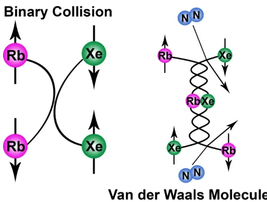
Figure 1.4: Spin exchange diagram showing the two possible means for polarization transfer between rubidium and xenon. Left: The polarized rubidium electron collides with the unpo-larized xenon nuclear and through a Fermi contact interaction the polarization is transferred to the xenon nucleus. The rubidium atom may again become polarized through optical pumping. Right: Formation and breakup of Rb-129Xe van der Waals molecules through three body collisions involving nitrogen. The interaction leaves the 129Xe polarized and the Rb depolarized.
molecule, the rubidium atom is left depolarized and will again absorb photons from the laser irradiation until it becomes repolarized.
also used for polarizing xenon, but the maximum achievable polarizations for xenon occur at low xenon partial pressures, meaning clinically relevant volumes (∼1 L) of highly polarized (>25%) xenon can be difficult to achieve using the batch method (Ben-Amar Baranga et al., 1998; Fink et al., 2005).
Fortunately, the spin exchange rates between xenon and rubidium are three orders of magnitude higher than between helium and rubidium, decreasing the pump-up time from hours to seconds and allowing xenon to be polarized via continuous-flow SEOP (Grover, 1978; Jau et al., 2003). In this method, a gas mixture including xenon, nitrogen, and helium are continuously flowed through the optical cell illuminated by laser light. Typically, a lean mixture of xenon (between 1% and 5%) is used to limit the spin destruction mechanism due to spin-non-conserving, binary, Rb-Xe collisions (Driehuys et al., 1996). The xenon gas atoms become polarized by SEOP with an optically thick alkali metal vapor, in the same way as the batch method, but continue to flow out of the cell where they are separated from the mixture and collected using a liquid nitrogen cold trap. Once the desired volume of xenon is frozen in the cold trap, the flow of gas is stopped, the optical cell is closed, and the polarized xenon is thawed and transferred to a storage container. Continuous-flow SEOP is the most widely used method for clinical applications as it offers the potential to produce large volumes of gas in a shorter amount of time than the batch method. The work presented here is completed exclusively using hyperpolarized xenon produced via continuous-flow SEOP.
Figure 1.5: Continuous-flow hyperpolarizer used for all work presented in this dissertation. Left: Schematic of the spin exchange optical pumping process in continuous-flow mode. Right: Our lab’s Polarean 9800 129Xe Hyperpolarizer which operates in a continuous-flow mode.
thawing for collection, and the larger volume of the spiral cold finger allows the xenon to freeze in a thin layer rather than a large chunk of ice. This leads to a decrease in solid state relaxation and prevents blockages in the flow during collection. The second variable part is the permanent magnet in which the cold finger is placed to increase the longitudinal relaxation of xenon while in the solid state. This magnet is interchangeable and our lab has two permanent magnet designs which may be used: the original magnet shipped with the polarizer and the magnet which is available in the Polarean 3777 129Xe Hyperpolarizer Upgrade Module. The original magnet has an open front for easy access to the liquid nitrogen dewar and a closed top which was used as a flux return. The new magnet design has a closed front and open top which generates a stronger and more homogeneous magnetic field which help produce larger final xenon polarizations.
1.2 Theoretical Model of Noble Gas Polarization
As polarization is transferred from the electrons of the alkali metal atoms to the nuclei of the noble gas, the noble gas polarization is directly related to the alkali metal polariza-tion. In the previous section, the process of spin exchange optical pumping was described qualitatively, but in this section, the polarization of 129Xe by spin exchange with optically pumped rubidium will be described quantitatively.
The theory behind spin exchange optical pumping of noble gas nuclei has been extensively studied and is fairly well understood (Happer, 1972; Walker & Happer, 1997). Following the work of Appelt et al. (1999b), Norquay et al. (2013), and Freeman et al. (2014), a theoretical model to determine the final 129Xe polarization during SEOP will be presented. The time dependence of the rubidium polarization throughout the length of the optical cell during optical pumping may be described by (Happer & Van Wijngaarden, 1987):
PRb(z, t) =
γOP(z)
γOP(z) + ΓSD
1−e−(γOP(z)+ΓSD)t (1.2.1)
where γOP(z) is the position-dependent Rb optical pumping rate with z representing the distance from the illuminated window of the optical cell, along its main axis and ΓSD is the rubidium spin destruction rate. This equation shows the exponential buildup of rubidium polarization. However, as the time needed to reach saturation of the Rb polarization is on the order of milliseconds while the time required for spin exchange is on the order of seconds or longer, the steady-state polarization of the rubidium can be used:
PRb(z, t) =
γOP(z)
γOP(z) + ΓSD
. (1.2.2)
Table 1.1: Spin destruction cross sections for Rb binary collisions
i κRb−iSD (cm3s−1)
Rb 4.2×10⁻¹³ (Ben-Amar Baranga et al., 1998) He 1.0×10⁻²⁹T4.26 (Ben-Amar Baranga et al., 1998) N2 1.3×10⁻²⁵T3 (Chen et al., 2007)
Xe 6.02×10⁻¹⁵ 298KT 1.17 (Freeman et al., 2014)
collisions (BC) with the various constituents of the gas mixture and the formation and breakup of van der Waals molecules (vdW). The contribution from binary collisions is given by:
ΓBCSD =X i
[Gi]κRb−iSD , (1.2.3)
whereκRb−iSD is the spin destruction cross section for rubidium binary collisions with each gas in the optical cell with an atomic density [Gi]. Table 1.1 lists the temperature dependent values for the spin destruction cross section of rubidium with the various gases present during continuous-flow SEOP.
The contribution of van der Waals molecules to rubidium spin destruction is dependent on temperature and the atomic gas densities of He, N2, and Xe (Ruset, 2005):
ΓvdWSD = 66183 1 + 0.92[N2]
[Xe] + 0.31 [He] [Xe] ! T 423K −2.5 (1.2.4)
As seen from this equation, to minimize the effects of the formation and breakup of van der Waals molecules on the rubidium spin destruction, it is advantageous to keep the xenon atomic densities low within the optical cell while maintaining high concentrations of nitrogen and helium. According to Equation 1.2.3, maintaining low xenon atomic densities also helps lower the spin destruction due to binary collisions while having high concentrations of nitrogen and helium have a negligible effect on binary collisions.
of ∆λl. The pressure-broadened D1 absorption cross section of rubidium will be modeled as a Lorentzian function. With these assumptions, the optical pumping rate, γOP, may be written (Appelt et al., 1999b; Antonacci et al., 2017):
γOP(z) =
β
[Rb]F, (1.2.5)
where F is the photon flux defined by F = I·np
A with I being the intensity of the pumping laser,np being the photons per Joule produced by the pumping laser, andAbeing the cross-sectional area of the pump laser as incident on the optical cell. [Rb] is the rubidium number density. It is important to note that when determining the rubidium number density within the optical cell most often vapor curves, such as those from Killian (1926), Nesmeyanov (1964), or Alcock et al. (1984), are employed along with the temperature reading from a resistance temperature detector (RTD) placed on the outside of the cell. This assumes that the rubidium vapor is in thermal equilibrium with a number density determined by an RTD on the outside of the optical cell and a uniform distribution along the entire length of the optical cell. The term β is defined by:
β = 2 √
πln2refD1λ3lw0(r, s)
hc∆λlnp
[Rb]. (1.2.6)
In this equation, re is the classical radius of the electron, fD1 is the rubidium D1 oscillator strength, h is Planck’s constant, andcis the speed of light. The function w0(r, s) is the real part of the complex overlap function dependent on r, the ratio of the atomic D1 linewidth to the pumping laser linewidth, and s, the relative detuning between the pumping laser and the D1 cross section (Appelt et al., 1999a).
Using the above equation, the attenuation of the optical pumping rate along the length of the optical cell may be described by:
dγOP(z) dz =−β
1−sz
γOP(z)
γOP(z) + ΓSD
wheresz is the fraction of laser photons that are circularly polarized. Equation 1.2.7 can be solved via separation of variables and provides a solution for the optical pumping rate such that (Appelt et al., 1999b):
[1 + (1−sz)(βz+K)]γOP(z) +γSDln(γOP(z)) +γSD(βz+K) = 0. (1.2.8)
K is a constant determined by the boundary condition at z= 0. γOP(0) is the initial optical pumping rate at z = 0 and forces the constantK to be:
K = −γOP(0) +γSDln(γOP(0))
γSD+ (1−sz)γOP(0)
. (1.2.9)
This solution for the optical pumping rate as a function of the z may be used to determine the optical pumping rate at discrete positions along the axis of the optical cell. Once the optical pumping rate is known for a specific position in the cell, it may be used to calculate the expected rubidium polarization at that point through Equation 1.2.2. This provides the ability to determine a mean rubidium polarization, hPRbi, throughout the cell which may be used to calculate the final xenon polarization. The xenon polarization is dependent on the residency time, tres, within the optical cell and exhibits an exponential buildup in polarization, similar to rubidium, described by (Driehuys et al., 1996):
PXe(tres) =
γSE
γSE+ Γ hPRbi
1−e−tres(γSE+Γ). (1.2.10)
total theoretical spin exchange rate to be calculated by (Cates et al., 1992):
γSE =γSEBC +γ vdW SE = κ
Rb−Xe SE +
X i|G1
i|
ξi
!
[Rb]. (1.2.11)
The spin exchange cross section due to binary collisions has been reported to be 2.2×10⁻¹⁶ cm3s−1 (Jau et al., 2003). The variable ξ
i is a van der Waals specific rate that has been measured for each gas atom in the mixture. The values have been calculated as ξXe =5230 Hz,ξN2 =5700 Hz, andξHe =17000 Hz (Cates et al., 1992; Zeng et al., 1985; Driehuys et al.,
1996).
The theory presented here is often used to make comparisons to experimental data for various polarizer designs and may be used for both batch method and continuous-flow SEOP. However, in all cases, the theory overestimates the polarization achieved experimentally by up to a factor of two. In the next section, the relaxation mechanisms of 129Xe which may lead to this discrepancy are reviewed.
1.3 Depolarization Mechanisms of Hyperpolarized Gases
Once 129Xe has been hyperpolarized, it is important to maintain the polarization up to the point it is put to use. This requires a thorough understanding of the longitudinal relaxation of xenon in the solid, liquid, and gas phases. Longitudinal relaxation, also known asT1 relaxation, involves the interaction of nuclear spins with the surrounding environment and, through energy exchange, causes the relaxation of a nuclear spin system back to thermal equilibrium. Here, the mechanisms which cause longitudinal relaxation of 129Xe in the gas and liquid phases are presented. The longitudinal relaxation rate may be described by the combined effects of multiple depolarization mechanisms using the following equation:
1 T1 = 1 T1 CR + 1 T1
In this equation, The relaxation has been categorized as collisional relaxation,CR, relaxation due to magnetic field inhomogeneities, M F I, and relaxation with molecular oxygen, O2. Collisional relaxation includes the intrinsic relaxation due to binary collisions and van der Waals molecules as well as the extrinsic relaxation caused by collisions with the container walls.
In the early stages of the development of SEOP, many of the intrinsic relaxation mech-anisms were studied. Hunt & Carr (1963) developed the theory on relaxation due to binary collisions through the identification of the spin-rotation Hamiltonian for the 129Xe nuclear spin. Relaxation resulted as magnetic fields were generated by the moving electrons in the xenon atoms during binary collisions. The highly polarizable xenon atoms are thus affected by these magnetic fields and may become depolarized. These magnetic fields are modulated by the lifetime of the collisions and thus have a small effect during the short lifetime of a binary collision. The formula for the relaxation rate of xenon caused by intrinsic binary collisions was determined to be (Streever & Carr, 1961; Hunt & Carr, 1963):
1
T1
= [Xe (amagat)]
56h·amagat (1.3.2)
While this equation was determined for xenon densities, [Xe], greater that 50 amagat, it was extrapolated down to ∼1 amagat, a regime much more relevant to SEOP, and predicts a T1 for xenon on the order of tens of hours. Therefore, in most SEOP polarizers these mechanism is ignored because, as will soon be shown, other relaxation mechanisms provide a much shorter longitudinal relaxation time on the order of tens of minutes.
Table 1.2: Room temperature coefficients, KB (×10−10 cm3/s), for the breakup of van der Waals molecules for xenon and nitrogen as measure by aChann et al. (2002) and bAnger et al. (2008).
Gas KB Xe 1.2a 3.7b N2 1.3a 1.9b
et al. (2008) provided an empirical formula for the relaxation rate caused by the formation of van der Waals molecules. When combined with Equation 1.3.2, the formula for the total intrinsic relaxation of 129Xe takes the form:
1
T1
= [Xe (amagat)] 56h·amagat +
1 4.59h
1 + 3.65×10⁻³B02
1 +rN2
[N2] [Xe]
−1
, (1.3.3)
whereB0is the applied magnetic field andrN2 is relative efficiency of nitrogen to breakup the
van der Waals molecules. The coefficients, KB, for the breakup of van der Waals molecules by xenon and nitrogen as measured by Chann et al. (2002) and Anger et al. (2008) are listed in Table 1.2. The relative efficiency of breakup, rN2, is given by rN2 =KB/KXe.
relaxation time of xenon up to 9 hours with no wall coating and very long lifetimes. This increase is helpful but in most cases a relaxation time due to wall collisions is expected to be on the order of tens of minutes to an hour. While optical cells used in batch method SEOP always make use of surface coatings, those used in continuous-flow SEOP forgo this costly procedure as the contribution from wall collisions to the longitudinal relaxation time is negligible because of the decreased residency time of the xenon atoms.
The contribution of relaxation due to magnetic field inhomogeneities is the subject of chapter 3 and as such will not be covered in detail here. However, it is worth noting that relaxation in magnetic field gradients is often ignored in continuous-flow SEOP even though it is possible to obtain relaxation times on the order of minutes in regions where the magnetic field approaches zero. However, with careful design of the continuous-flow SEOP setup, relaxation arising from diffusion in magnetic field gradients can be increased to tens of minutes or hours.
Finally, relaxation through interactions with oxygen is one of the strongest longitudinal relaxation mechanisms of hyperpolarized xenon owing to the permanent magnetic dipole moment of oxygen. During SEOP and transport, depolarization of xenon because of interac-tions with molecular oxygen can be minimized by flushing the leak-proof storage container several times with ultra-high purity nitrogen gas before use. Unfortunately, interactions with oxygen become unavoidable duringin vivo experiments with 129Xe. Experiments performed to measure the relaxation arising from collisional coupling of oxygen produced a formula for the relaxation rate described by (Jameson et al., 1988):
1
T1
= 0.478s−1amagat−1
nO2. (1.3.4)
In this equationnO2 is the oxygen density. This equation reveals that at atmospheric
1.4 Overview of Contents
In this dissertation, work fundamental to the understanding of continuous-flow spin exchange optical pumping inefficiencies is presented.
In chapter 2, the fluid flow within optical cells used for continuous-flow SEOP is studied. Previous work has been done to simulate flow within the optical cell but multiple assumptions and symmetries are used to simplify the simulations. These assumptions ignore important aspects which can considerably affect the fluid flow. Work simulating the entire 3D geometry of two different optical cell designs is presented. This work suggests that the path the gas takes before entering the optical cell influences gas flow within the optical cell and that turbulence is introduced at much lower flow rates than expected, close to those flow rates used for production of clinically relevant doses of hyperpolarized gas. Additionally, this turbulence leads to a distribution of residency times, antithetical to the way that the residency times are treated when modeling xenon polarization. These results could explain the discrepancy found between theoretical and experimental polarization levels achieved during continuous-flow SEOP.
In chapter 3, the contribution of gas diffusion in magnetic field inhomogeneities to the depolarization of xenon during continuous-flow SEOP is discussed. Through the combined use of finite element analysis and random walk simulations, large gradients were discovered in the flow path of the gas that can lead to a significant increase in the longitudinal relaxation rates of hyperpolarized 129Xe, particularly in regions where the magnetic field approaches zero. The results were validated using experimental longitudinal relaxation measurements of two different permanent magnet designs, generating significantly different magnetic field distrubutions. The work suggests that careful design of the magnets required for continuous-flow SEOP can minimize the effects of magnetic field gradients on longitudinal relaxation, leaving wall collisions as the largest remaining source of gas phase spin relaxation during SEOP of xenon.
SPIONs is analyzed and used as a new source of contrast in magnetic resonance imaging. Specifically, the effects of longitudinal and transverse spin relaxation are separated and characterized for hyperpolarized 129Xe undergoing restricted diffusion near SPIONs using finite element analysis and Monte Carlo simulations. Simulations showed that signal loss near the SPIONs is almost entirely caused by transverse relaxation with only a small contribution from longitudinal relaxation. Simulated image contrast and experimental images revealed that xenon diffusion provides no noticeable increase in sensitivity to SPIONs at the length scales typically probed by MRI. This indicates that to increase image contrast near iron oxide nuclei with larger gyromagnetic ratios and/or diffusion coefficients, such as 3He or fluorinated gases, should be used.
CHAPTER 2: CHARACTERIZATION OF FLUID FLOW IN CONTINUOUS-FLOW SPIN EXCHANGE OPTICAL
PUMPING CELLS
In this chapter, results from an investigation into the fluid flow within optical cells used for continuous-flow spin exchange optical pumping of129Xe gas are presented. Wall collisions are known to be a significant source of relaxation for hyperpolarized xenon gas. Designing cells that generate laminar flow and minimize contact with the cell walls are necessary to achieve maximum polarization. Computational fluid dynamics and heat transfer simulations are performed on two different optical cells designed for use in a commercial hyperpolarizer to determine the flow regime inside the cells. These simulations reveal turbulence in both designs at flow rates typically used to generate clinical volumes (∼1 liter) of hyperpolarized 129Xe. This turbulence leads to a wide distribution of residency times for xenon in the optical cell which could contribute partially to the discrepancy between the predicted and experimental polarization levels currently achieved.
2.1 The Discrepancy between Theoretical and Experimental Nuclear Spin Po-larization of 129Xe
resonance experiments to measure the rubidium polarization profile during continuous-flow SEOP. They concluded that, at least for their system based on the polarizer design from Ruset et al. (2006), the rubidium polarization was between 85% and 95%. As the rubidium polarization directly affects the xenon polarization, another mechanism must be causing the discrepancy. Antonacci et al. (2017) used atomic absorption spectroscopy to measure polar-ization losses due to dark rubidium vapor in the outlet of the optical cell. They found that dark rubidium also has a negligible impact on the final xenon polarization under typical ex-perimental conditions. Even correcting the theoretical model to incorporate the combination of all of these effects cannot account for the nearly factor of two difference often observed between theoretical and experimental xenon polarizations.
This has led to the hypothesis that perhaps there are factors missing from the theoretical model of xenon polarization. Freeman et al. (2014) have proposed the presence of paramag-netic rubidium nanoclusters in the cell during SEOP. The presence of rubidium nanoclusters would fundamentally change the theoretical framework of xenon polarization. By including the production of these particles and the depolarizing effects they have into the standard theoretical model of spin exchange optical pumping, they were able to show consistency between the predicted and observed xenon polarization levels. However, while Flower et al. (2017) used electron microscopy to observe rubidium particles in certain locations of some optical pumping cells, these experiments were not performed during SEOP and no exper-imental evidence has yet shown the presence of rubidium clusters during continuous-flow SEOP. Until such time as these clusters are shown to be present during SEOP, the culprit behind SEOP inefficiency is still unknown.
spin exchange that are still used today, including the need to presaturate the gas mixture with rubidium vapor prior to entering the optical cell and to preheat the gas to the oven temperature to avoid temperature gradients leading to turbulent flow. Unfortunately, the simulations performed by Fink & Brunner (2007) used simplified optical cell geometries that neglect the complex flow that develops before the gas enters the main body of the cell. In addition, assumptions about the rubidium density distribution within the optical cell are made which are possibly incorrect for many polarizers.
In the work presented here, a systematic approach is taken to determine the factors that most affect fluid flow within the optical cell during continuous-flow SEOP. This is accomplished by performing computational fluid dynamics simulations on two, complete, full-scale optical cell designs for the only available commercial hyperpolarizer. The effect of using a plug flow versus a fully-developed flow is simulated along with the effect of a density-dependent gravitational force on the gas. The fluid dynamics equations are then coupled with the heat equation to understand the effect of convection on the fluid flow within the two optical cell designs. Finally, a model of rubidium evaporation is included to determine the effect of heat absorption caused by the latent heat of vaporization. Comparisons to previous experimental work are used to test the accuracy of these simulations.
2.2 Optical Cell Designs
used in our system is composed of 1% xenon, 10% nitrogen, and 89% helium by volume. During operation, the gas is typically flowed at a volume rate between 0.1-1.5 SLM and a total pressure of 2 atm. The optical cell, housed within the temperature-controlled oven, is maintained at a temperature of 408 K while the temperature of the presaturation region is controlled via wraparound heating cord to 458 K.
Figure 2.1: SolidWorks models of both cell designs simulated in this investigation. Left: Older cell design with a presaturation “bulb” before the inlet, which is at the rear of the optical cell. Right: Newer cell design with inlet at the bottom of the cell. The presaturation region is still present but is no longer a bulb.
2.3 Computational Fluid Dynamics Simulations of Flow within the Optical Cell
2.3.1 Plug Flow and Fully Developed Flow at the Cell Inlet
According to the theoretical model of xenon polarization, the polarization level is de-pendent on the residency time of xenon within the optical cell. The longer the spins spend within the optical cell, the greater the final polarization that is achieved. Therefore, the average residency time can help to estimate the maximum achievable xenon polarization. Typically, to calculate the residency time within the cell, τres, the volume flow rate is used in the following manner:
τres =
V
Q, (2.3.1)
where V is the volume of the optical cell and Q is the volumetric flow rate. Underlying this method of calculating the residency time are a number of assumptions. The flow profile in the cell is assumed to be radially uniform meaning all atoms have the same speed. This is a poor assumption in the case of continuous-flow SEOP as there is a great deal of piping before the optical cell which will lead to a fully developed flow profile entering the cell. Additionally, using the average residency time based on the flow rate assumes that there is no turbulence present in the optical cell. Turbulence could lead to a wide range of xenon residency times vastly changing the final xenon polarization. Computational fluid dynamics simulations by Fink & Brunner (2007) have already revealed turbulence in a simplified model of continuous-flow optical cells indicating that assuming laminar flow within complex optical cell designs is likely incorrect.
Figure 2.2: The development of the velocity profile in a pipe. The flow enters the pipe as a plug flow then after the necessary entrance length becomes fully developed. The fully developed velocity profile has a parabolic shape.
increases to maintain the mass flow rate through the pipe. Therefore, a velocity gradient develops along the pipe. A certain entrance length is required for the flow to develop this velocity gradient. After the entrance length, the flow is said to be fully developed. Figure 2.2 shows a developing flow within a pipe. As can be seen, magnitude of the velocity at the boundary is zero, while the speed at the center is twice the velocity at the inlet.
For all simulations, a k-ω turbulence model was employed in solving the Reynolds-averaged Navier-Stokes equations in three dimensions using a stationary solver (Bassi et al., 2005). The k-ω turbulence model was chosen because of the low Reynolds number of the conditions simulated. Modified versions of both cells were designed without the inlet portion to simulate the plug flow at the inlet of the of the main body of the optical cell and are shown in Figure 2.3. In order to simulate a fully developed flow at the inlet of the optical cell, inlet conditions were obtained from a separate simulation to generate a fully developed flow profile. Owing to the symmetry of the pipe flow, a 2D axisymmetric simulation was used. The pipe had a diameter of 7.84 mm to match the inlet diameter of the optical cell and was taken to be 200 diameters long to ensure the flow was truly fully developed at the outlet. The inlet conditions were taken to be plug flow profiles with velocities of 0.1296 m/s, 0.2592 m/s, 0.3888 m/s, and 0.5184 m/s corresponding to volume flow rates of 0.375 SLM, 0.75 SLM, 1.125 SLM, and 1.5 SLM, respectively. These flow rates were chosen as they are values typically used to generate pre-clinical and clinical volumes of HP129Xe using continuous-flow SEOP. An example of the velocity profile at the inlet for plug flow and fully developed flow is shown in Figure 2.4
After performing the 2D axisymmetric simulations, the outlet results for the velocity, turbulent kinetic energy (k), and specific dissipation rate (ω) were mapped onto the inlet boundary condition for the 3D simulations. A normal inflow boundary condition was used at the inlet when simulating a plug flow for the four different flow rates simulated here. The temperature of the gas was kept constant at a typical oven temperature of 408 K for all simulations. A force was included on the fluid volume to determine the effect of gravity on the flow. This was accomplished through the use of a force in the negative z-direction as indicated in Figure 2.5 based on the local gas density and a parameterized gravitational constant that was taken to be zero or 9.81 m/s2 to turn gravity off or on.
Figure 2.3: SolidWorks models of both cell designs used to simulate plug flow at the inlet of the main cell body. Left: Older cell design with inlet leg removed where the boundary condition at the rear of the cell was taken to be an inlet with a normal inflow velocity whose magnitude was the average velocity for a given flow rate. Right: Newer cell design with inlet leg removed. Boundary condition was again taken to be an inlet with a normal inflow velocity.
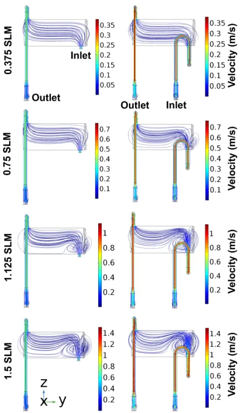
both cases, but the flow rate at which turbulence is introduced is not the same. For the fully developed flow simulations, turbulence is introduced as early as 0.75 SLM while turbulence begins around 1.125 SLM in the case of a plug flow. The figure also shows that the flow field in the case of the plug flow looks quite similar to the fully developed flow at a lower flow rate. For example, the flow field for a plug flow at 1.125 SLM looks much like the flow field for the fully developed flow at 0.75 SLM. This indicates that when assuming a plug flow during modeling of xenon polarization, the residency time may be estimated incorrectly because of turbulence increasing the residency time for some atoms while decreasing the residency times for others.
Figure 2.4: Comparison of plug flow velocity profile to fully developed flow velocity profile for flow rate of 1.5 SLM. Left: Plug flow velocity profile showing a uniform velocity of 0.5184 m/s corresponding to the 1.5 SLM flow rate. Right: Fully developed velocity profile exhibiting the expected shape and values. The velocity at the center is twice the velocity at the inlet and the gradient is parabolic with a velocity of zero at the boundary.
transfer was not included in these simulations meaning the temperature throughout the cell was uniform leading to the absence of convection within the cell. While the streamlines are helpful in gaining some knowledge about the flow in the cell they do not provide quantitative information on the time individual particles spend in the optical cell.
Particle tracing simulations were performed in all fully developed flow cases to determine the residency time of xenon in the optical cell. Xenon molecular mass and diameter were specified as particle properties for the particles in the simulation. Temperature, pressure, velocity field, and dynamic viscosity results from the turbulent flow and heat transfer sim-ulations were used to include a drag force on the particles. Particles were released with a density proportional to the velocity magnitude at the inlet. A total of 5000 particles were released at time zero and a time-dependent solver was employed to determine each particle’s position and velocity every tenth of a second up to a total time of 60 seconds. The particles underwent an elastic collision if they interacted with the wall except at the outlet. A freeze condition was taken at the outlet boundary in order to allow solution of an auxiliary variable which determined the total residency time of each particle.
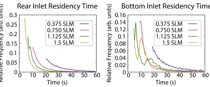
Figure 2.6: Histogram plots showing relative frequency of the residency time for each second in the optical cell for both cell designs at all simulated flow rates. Partitions are connected by lines to more easily show temporal trends. Left: Residency times for the older cell design with the outlet at the rear of the cell. The smooth, exponentially-decreasing shape of the plot shows the lack of turbulence in the cell Right: Residency times for the new cell design with the outlet at bottom of the cell. For the 1.125 SLM and 1.5 SLM plots, the spikes are indicative of significant turbulence affecting the residency times.
cell for various geometries, inlet velocity profiles, and flow rates, they are not yet a complete picture of the hydrodynamic and thermodynamic processes occurring during SEOP.
2.3.2 Effects of Convection on the Flow Field within the Optical Cell
The effect of convection on the flow was determined by coupling the heat equation to the Navier-Stokes equations within COMSOL Multiphysics to simulate the heat from the oven and heat from the wraparound heating cord on the presaturation region. The CAD models were modified to include an additional material domain which served as the PYREX (Corning Inc., NY, U.S.A.) portion of the optical cell. For these simulations, all boundary condition from the CFD models remained the same. As the gas was not preheated before entering the cell, the boundary condition at the inlet was taken to be a constant temperature of 293 K to match the ambient temperature in the laboratory. The boundary condition for the presaturation region of each cell was a constant temperature of 458 K to simulate heat transfer from the heating cord, which was temperature controlled via resistance temperature detector on the glass surface, wrapped around the region. All other boundaries were given a heat flux boundary condition at a temperature of 408 K to simulate the convection on the external walls of the optical cell from the oven in which the optical cell was housed.
of the flow field. Both gravity and convection did not lead to turbulence in the older cell design even at 1.5 SLM.
Figure 2.7: Flow field within the optical cell at 0.375 SLM when conduction and convection are included in the simulations. Top: Flow field in the bottom inlet optical cell. The gravitational force creates turbulence when convection is included at the lowest flow rate tested which was not the case in the absence of convection Bottom: Flow field in the rear inlet optical cell. Whether the gravitational force is included or not the flow remains qualitatively the same. This was true for all flow rates tested for this cell design.
2.3.3 Modeling Rubidium Vaporization within the Presaturation Region
To incorporate heat loss from rubidium vaporization, a rubidium evaporation model was included in the simulations. The CAD models were again modified to include a pool of liquid rubidium, colored red in Figure 2.8, at the bottom of the presaturation region for each cell. The rubidium pool was 13.8 mm wide by 15.4 mm long for the optical cell with the inlet at the rear of the cell and 4.3 mm wide by 29.9 mm long for the optical cell with the inlet at the bottom of the cell. A boundary heat source for the latent heat of vaporization was used as the boundary condition for the rubidium/gas mixture boundary. The value of the heat source was calculated using the latent heat of vaporization for rubidium and a modified version of the Hertz-Knudsen equation:
φq =
−Hvap
NA
α(psat) √
2πMRbkBT
, (2.3.2)
whereHvap is the specific heat of vaporization of rubidium (844.95 kJ/kg),NA is Avogadro’s number, α is the sticking coefficient of the rubidium gas, MRb is the molecular mass of rubidium in kilograms, kB is the Boltzmann constant, T is the local temperature, and psat is the saturation pressure of rubidium taken from the vapor pressure curve. The sticking coefficient is taken here to be 1 in order to calculate a best-case scenario rubidium evaporation and because the value is expected to be near unity (Nagayama & Tsuruta, 2003; Tsuruta et al., 1999). The partial pressure of rubidium has been removed from the Hertz-Knudsen equation to simplify computation of a steady state solution. All other boundary conditions for heat transfer were kept the same for these simulations.
Figure 2.8: Modified SolidWorks models of both cell designs with the addition of rubidium in the presaturation region. Left: Older cell design with rubidium in the presaturation “bulb” before the inlet. Right: Newer cell design with rubidium in the presaturation region below the cell inlet.
Figure 2.9: Flow field within the optical cell at 1.5 SLM for the optical cell with the inlet at the rear Left: Flow field when heat conduction and convection are included in the simulation but rubidium vaporization is neglected. No turbulence is present in the cell Right: Flow field when heat conduction, convection, and heat loss due to rubidium vaporization are included in the simulation. Notice that turbulence occurs in this case and that the gas preferentially moves to the right side of the cell.
for the rear inlet cell design, this turbulence is not noticeable on the residency time plots as shown by the smooth nature of the curve. In the case of the bottom inlet cell design, the turbulence is now noticeable at a flow rate of 0.75 SLM. The average residency time for all flow rates in both optical cell designs has decreased as compared to Figure 2.6 because of the increase in particle speed. The average residency time at a flow rate of 1.5 SLM is 4.9 s for the rear inlet cell and 8.6 s for the bottom inlet cell, both of which are shorter than the plug flow prediction of 10.8 s.
Figure 2.10: Histogram plots showing relative frequency of the residency time for each second in the optical cell for both cell designs at all simulated flow rates with heat conduction, convection, and rubidium vaporization included. Partitions are connected by lines to more easily show temporal trends. Left: Residency times for the rear inlet cell design. While streamlines show turbulence in the cell at the higher flow rates, the histogram does not reveal this turbulence. It is important to note that at 1.5 SLM nearly 100% of the particles have already left the cell in under 10 s. Much shorter than the time required for spin exchange to occur. Right: Residency times for the bottom inlet cell design. Turbulence in the cell can be seen at flow rates of 0.75 SLM, 1.125 SLM, and 1.5 SLM as indicated by the bimodal shape of the histogram.
for the expected xenon polarization to reach 63% of its maximum possible value. It can be defined using the xenon spin exchange rate, γSE, and the xenon spin destruction rate, Γ, in the following manner (Freeman, 2015):
τSU = 1
γSE+ Γ
. (2.3.3)
increases.
These simulations still do not provide a complete picture of fluid flow during continuous-flow SEOP. Heating from laser radiation incident on the front of the cell has not been added to these simulations. While the addition of laser heating is important to accurately measure the most realistic average residency time based on flow rate, temperature, and cell geometry, the shape of the flow field is not expected to change drastically when laser heating is included. In the work performed by Antonacci et al. (2017), video was taken of the fluid flow inside the cell when the laser was turned on and the flow of the particles matches qualitatively with the results achieved in the work presented here. Of course, this is not definitive proof of the veracity of the simulations, but it does appear to point to the laser heating having less effect on the shape of the flow field and more likely increasing the speed of the particles because of increased temperature.
2.4 Conclusions
These simulations revealed that using a plug flow velocity profile at the inlet of the optical cell incorrectly determines the flow field inside the cell for a given flow rate. As such, a fully developed velocity profile must be used at the inlet to accurately determine the velocity field inside the cell. It was also shown that turbulence in the cell could lead to longer average residency times for xenon compared to laminar flow at high flow rates. This means optical cells that exhibit turbulent flow may actually lead to higher xenon polarizations through xenon spins spending a longer amount of time in the region where spin exchange can occur. When heat transfer was added to the simulations, the results indicated that gravity can create convection rolls that lead to turbulence, even at flow rates that did not show turbulence when the temperature was uniform. Including this effect is therefore necessary to determine an accurate flow field inside the optical cell. Heat loss due to rubidium vaporization played a significant role in the flow for the higher flow rates. The heat loss led to temperature gradients in the presaturation bulb of the cell designed with the inlet at the rear of the cell. This turbulence then propagated to the main body of the cell which did not contain turbulence at any of the flow rates tested when rubidium vaporization was not included.
This work suggests that a possible cause for the discrepancy between theoretical and experimental polarization levels is the low residency time for many atoms in the optical cell. Obviously, one option to increase residency time would be to flow the gas at a lower flow rate. However, this is not possible for most clinical applications which are time-sensitive and require multiple batches of HP129Xe. Another option would be to design an optical cell with increased turbulence such that recirculation in the cell would lead to larger residency times. This would be problematic as wall collisions with the cell could lead to significant spin destruction in that case. Therefore, it appears that longer optical cells with larger volumes are necessary to increase the residency time of xenon within the main body of the cell to provide sufficient time for spin exchange to occur.
CHAPTER 3: HP 129Xe DEPOLARIZATION IN MAGNETIC FIELD GRADIENTS DURING CONTINUOUS-FLOW SEOP 1
In this chapter, results from an investigation on the effect of diffusion-mediated 129Xe gas depolarization in magnetic field gradients during continuous-flow SEOP is presented. A combination of finite element analysis and Monte Carlo simulations is used to determine the effect of these gradients for the first generation of a commercial, continuous-flow xenon polarizer, while experiments are performed to validate these simulations. The results here show that large gradients in the gas-flow-path can have a significant effect on the longitudinal relaxation of hyperpolarized 129Xe, especially in regions where the magnetic field assumes negligible values. To this end, care should be taken in the design of the permanent magnets required for continuous-flow SEOP. In the absence of such gradients, wall collisions are the major contributing factor to gas-phase spin relaxation of HP 129Xe.
3.1 Effect of Magnetic Field Gradients on 129Xe Depolarization
Early on in the lifetime of two of the most prominent hyperpolarization techniques for noble gases (metastability exchange optical pumping and spin exchange optical pumping), much work was being done to determine the effects of the various longitudinal relaxation mechanisms which depolarize the noble gas. Gamblin & Carver (1965) and Schearer & Walters (1965) were working simultaneously, albeit independently, to characterize the newly identified longitudinal relaxation mechanism of diffusion through magnetic field gradients. In order for the gas to remain polarized while moving in a magnetic field gradient, it is
1The work presented in this chapter was originally published in the Journal of Magnetic Resonance, see
essential that the gas does not violate the adiabatic condition:
1
B0
dBT dt
γB0, (3.1.1)
with γ being the gyromagnetic ratio of the diffusing spin and BT being the transverse com-ponent of the of the local magnetic field B0. If this condition is violated the nuclear spins will be unable to “follow” the field, resulting in their depolarization. Cates et al. (1988) extended the work done by Gamblin & Carver (1965) and Schearer & Walters (1965) by characterizing the effect of magnetic field gradients on the longitudinal relaxation of noble gases at low pressure.
Gradient-induced spin relaxation has also been studied for hyperpolarized129Xe gas near the fringe field of superconducting magnets but is often ignored during continuous-flow SEOP (Zheng et al., 2011). While most batch-mode polarization systems contain one or more sets of Helmholtz coils to generate a low (tens of gauss), uniform magnetic field necessary for SEOP, continuous-flow polarization systems contain an additional magnet used to generate a much higher magnetic field (kilogauss) in which the frozen gas is stored during the collection process. Depending on the relative configuration of these two magnets, the probability that the polarized gas, while traveling from the optical cell contained within the low field to the cold trap contained within the high field, flows through a region where the magnetic field rapidly changes direction and violates the adiabatic condition is particularly high.
3.2 Theoretical Background
The contribution of magnetic field inhomogeneities to the longitudinal relaxation of hyperpolarized gases is well described by the following relation (Gamblin & Carver, 1965; Schearer & Walters, 1965):
1
T1
=D|∇Bx|
2
+|∇By|2
B2 0
1 + Ω20τc2−1. (3.2.1)
In this equation, D represents the diffusion coefficient of the hyperpolarized gas and the mean magnetic field,B0, is assumed to lie along a well-defined quantization axis (taken here to be the z-axis). Bx andBy represent the transverse components of the magnetic field while |∇Bx| and |∇By| are their spatial gradients. In this case, the spatial gradients are assumed to be independent of position (Cates et al., 1988). The extra factor, (1 + Ω20τc2)−1, known as the magnetic-decoupling factor, accounts for rotation of spins between kinetic collisions, where Ω0 is the Larmor frequency andτc, the diffusion correlation time, is the time between collisions. As can be seen in Figure 3.1, this factor for 129Xe is nearly unity for a mean magnetic field below 20T, much higher than the magnetic fields used in this work, and will be omitted.
The assumptions in Equation 3.2.1 may be valid within the optical pumping cell, which is contained within the polarizing field generated by a Helmholtz coil, but they are not valid when the gas flows out of this region, where the magnetic field is on the order of a few tens of gauss, to the liquid nitrogen cold trap, where the magnetic field is on the order of thousands of gauss. Therefore, a modified version of Equation 3.2.1 which removes these assumptions is necessary:
1
T1
=D|∇BT|
2
B2 0
. (3.2.2)
0.9996 0.99965 0.9997 0.99975 0.9998 0.99985 0.9999 0.99995 1
0 5 10 15 20 25 30
Magnetic-decoupling Factor (1)
Field Strength (T)
129
Xe
3
He
Figure 3.1: Plot of the magnetic-decoupling factor as a function of magnetic field strength for 129Xe and 3He. The value for 129Xe is very nearly 1 for the magnetic field strengths presented in this work.
field along a well-defined quantization axis, it is important to note that a large relaxation rate in Equation 3.2.2 can be obtained whenever the magnetic field rapidly changes direction and assumes very low values, like in the case of a zero-field crossing. All results presented here will utilize Equation 3.2.2.
3.3 Simulating Depolarization of 129Xe Gas in Magnetic Field Gradients
3.3.1 Magnet Designs and Models
All work presented here was performed on a Polarean 9800129Xe Hyperpolarizer system (Polarean Inc., Durham, NC, U.S.A.), a system currently used by several research groups around the world. In this system, a single pair of Helmholtz coils creates the polarization field, while the holding field is created by an interchangeable permanent magnet composed of steel and rare-earth magnets. A full-scale model of the setup was developed using the computer-aided design (CAD) software SolidWorks (Dassault Syst`emes SolidWorks Corp., V`elizy-Villacoubly, France) as shown in Figure 3.2.
Figure 3.2: 3D model of the continuous-flow SEOP setup used in this work. The model includes the Helmholtz coil, the optical cell, the cold finger, and the interchangeable per-manent magnet and frame (highlighted in blue). The interchangeable perper-manent magnet allowed for an easy change to the distribution of the magnetic field in the region in which the gas diffuses after thawing (colored in red). North (N) and South (S) magnetic poles have been labeled to show the direction of the magnetic field.